Incorporating Machine Learning in Capture-Recapture Estimation of Survey Measurement Error

1 Introduction

There is increasing demand and interest in using nonprobability-based data sources and machine learning within fields such as survey research, official statistics, or economic and social sciences (De Broe et al., 2021; Galesic et al., 2021; Puts & Daas, 2021). Beaumont (2020) identified five causing key factors: declining survey response rates, high data collection costs, increased response burden, the desire for access to real-time statistics, and the growing availability of nonprobability data sources. However, using non-probability data and machine learning is still largely considered experimental in official statistics production (Beck, Dumpert, & Feuerhake, 2018; Braaksma & Zeelenberg, 2020). To use non-probability data in official statistics, Klingwort, Buelens, and Schnell (2019) proposed linking non-probability data with probability-based survey data to quantify survey measurement error by applying capture-recapture (CRC) techniques. CRC estimation is typically used to estimate an unknown population size. For instance, suppose 50 fish are caught from a pond. All are marked and released again. If 40 fish are recaptured, 10 of which are marked, then the simplest CRC estimate of the number of fish in the pond is

. The method’s applicability in estimation of survey measurement error has been confirmed by an additional in-depth study (Klingwort, Burger, Buelens, & Schnell, 2021). The exact methodology will be explained in Sect. 4.

Given the high-quality standards for official statistics (Eurostat, 2017), assessing how consistent these results are over time is required. Furthermore, the proposed CRC estimators were based on generalized linear modeling. This paper will study whether a machine learning algorithm provides better predictions, resulting in more precise quantifications of the survey measurement error.

The paper is organized as follows. Sect. 2 provides the research background of this study. Sect. 3 describes the data used in this paper. Sect. 4 describes the methodology, including CRC assumptions, generalized linear modeling, machine learning algorithms, model selection, model performance, and variance estimation. Results are presented in Sect. 5. Sect. 6 contains a discussion, and Sect. 7 concludes the paper.

2 Research Background

Diary surveys, for example, those that require each participant to report over multiple days, are among the surveys with the largest response burden. To reduce the response burden, respondents may respond inaccurately or not at all. As a result, estimates may be biased and precision may be compromised (Ashley, Richardson, & Young, 2009; Krishnamurty, 2008; Richardson, Ampt, & Meyburg, 1996). These errors fall under measurement and nonresponse errors in the Total Survey Error Framework (Biemer, 2010). Weighting techniques are usually applied to correct selective nonresponse. However, quantifying and correcting the measurement error is often impossible due to the absence of external sources for validation. Klingwort et al. (2019) proposed using CRC to quantify the measurement error by linking non-probability road sensor data to the Dutch Road Freight Transport Survey. The proposed CRC estimators correct for both nonresponse and measurement error, while the survey estimate is corrected for selective nonresponse only. The difference between the CRC and survey point estimates can be attributed to measurement error. A likely explanation for this difference is underreporting in the survey, given the high response burden (Klingwort et al., 2021).

The proposed methodology by Klingwort et al. (2019) is based upon well-established CRC estimators proposed by Alho (1990), Fienberg (1972), Huggins (1989), Lincoln (1935), and Petersen (1893). The model-based CRC estimators use covariate information to improve the estimate’s accuracy. For these models, logistic regression and log-linear models are used. In this paper, we study whether a machine learning algorithm will provide better predictions than the statistical models and how this affects the estimation of survey measurement error.

Breiman (2001) identified two cultures in statistical modeling: one is focused on explanation by assuming stochastic relationships between input and output (e.g. generalized linear models), whereas the other is focused on prediction without making these explicit assumptions (e.g. machine learning). Machine learning algorithms have several advantages over stochastic data models. They are more effective and efficient in mapping complex, nonlinear relationships and interactions between auxiliary information and a target variable in a high-dimensional feature space (Boulesteix & Schmid, 2014; Grimmer, Roberts, & Stewart, 2021; James, Witten, Hastie, Tibshirani, & Taylor, 2023). In addition, some machine learning algorithms, such as gradient boosting, are less sensitive to multicollinearity and can handle missing values naturally. Machine learning has gained momentum by the increase in digital data and improved hardware and open software. Note that there is some confusing terminology used by the two cultures: (multinomial) logistic regression is a data model that is applied to a categorical outcome variable, whereas in machine learning the term regression is reserved for a numeric outcome variable.

The current state of research on using machine learning for CRC is very limited. Whytock et al. (2021) applied machine learning to estimate species occupancy from camera trap data. Rankin (2017) introduced statistical boosting for an open-population CRC model, allowing for automatic feature selection and including non-linear effects (an open population means that the population size may change during the study period as a result of births, deaths, immigration, or emigration). Yee, Stoklosa, and Huggins (2015) applied vector generalized additive models (VGAMs) to capture-recapture data, which are a nonlinear extension of commonly used parametric approaches. The current study demonstrates a novel empirical application of machine learning for CRC estimation for closed populations within the context of official statistics and survey research.

Moreover, the study by Klingwort et al. (2019) was based upon one year of data. To better understand the proposed method, it is required to assess how consistent the conclusions are over time. This is particularly important concerning the quality of the non-probability data (Carciotto & Signore, 2021). As will be shown, the sensor data quality is declining considerably over time, and whether this affects the estimated survey measurement error will be studied.

3 Data

3.1 Survey data

The Road Freight Transport (RFT) survey is a mandatory self-administered diary survey conducted by Statistics Netherlands providing statistics on Dutch commercial vehicles¹ at quarterly and annual intervals (Eurostat, 2016). The target population is the Dutch commercial vehicle fleet, excluding military, agricultural, and commercial vehicles older than 25 years. Furthermore, only vehicles weighing at least 3.5 tons and at least 2 tons of load capacity are considered. Stratified random samples are drawn quarterly from the vehicle register. A sampling unit consists of a vehicle license plate and a specific week. The owner of a sampled vehicle is assigned a week for which he or she has to report the days the vehicle was used. Therefore, this study’s target variable is defined as the number of vehicle days (D). One vehicle day is defined as a day a vehicle has been on the road for transport purposes in the Netherlands.

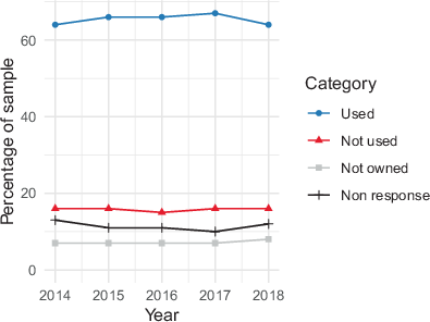
The respondents could report per day whether the vehicle was used or not used. It was possible to respond that the vehicle was not owned. Those that did not respond were categorized as nonresponse. For this study, the response category not owned is defined as frame error and excluded from the analysis to avoid false-positive links. Reasoning and potential effects are discussed by Klingwort et al. (2021). Moreover, the nonresponse units are also excluded from the analysis, and the survey weight is used to correct for the nonresponse. This choice is different from the earlier studies, in which the CRC estimators ignored the survey weights and treated nonresponse as reported ‘not used’ (Klingwort et al., 2019; Klingwort et al., 2021). The distribution of response categories is comparable over the years (Fig. 1). Vehicles reported ‘not owned’ were considered a frame error and excluded from the response. Considering them as nonresponse error slightly decreases the relative difference between survey and CRC estimate (Klingwort et al., 2021). After excluding not-owned vehicles, the sample size was about 32 thousand per year.

Fig. 1 RFT survey response categories (%) per year

3.2 Sensor data

Sensor stations (Weigh-in-Motion, WiM) on Dutch highways continuously weigh every passing vehicle while registering the license plate and timestamp. The license plate and timestamp registration are important for this study, as they allow for the deterministic record linkage with the survey and administrative data. The sensor system consists of nine stations permanently installed in both directions on Dutch highways, resulting in 18 sensor stations. Fig. 2 shows the daily number of working sensors. In 2014 and 2015, most of the sensors were operating and continuously measuring. This number decreased beginning in 2016. In 2017, hardly any stations were active, and there were even days without working sensors. At the beginning of 2018, more sensors were recording again but still considerably fewer than in previous years. This measurement inconsistency poses concerns about whether the proposed methodology by Klingwort et al. (2019) is robust against a decline in the quality of the nonprobability data because the initial study was based on data from 2015, the year with the most consistently working sensors.

Fig. 2 Daily number of working sensors between 2014 and 2018

3.3 Register data

The Vehicle Register (VR) and the Business Register (BR) provide additional administrative data with information about technical vehicle characteristics and vehicle owners, respectively. The VR contains 16 covariates like vehicle equipment class, emission class, the maximum mass of the vehicle, the mass of the empty vehicle, loading capacity, the status of the owner (person or company), province where the owner is located, and vehicle classification. The BR contains six covariates, examples being the classification of economic activity (NACE), classification of company size, and the size of the vehicle fleet. For a complete list with further details, we refer to Klingwort (2020).

3.4 Data linkage

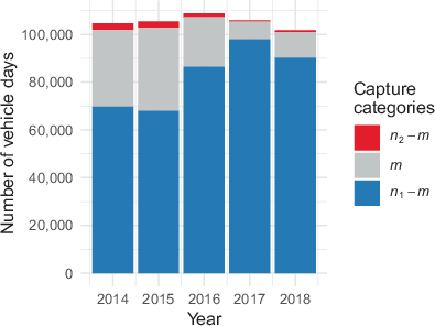
The RFT survey response data, WiM sensor data, and VR and BR administrative data were linked on micro-level: the survey response and sensor data by license plate and date; the VR and BR data by license plate, year, and quarter. After linkage, contingency tables with the number of vehicle days can be constructed per year. Cells include n₁ denoting the weighted number of vehicle days reported used in the survey, n₂ denoting the weighted number of vehicle days detected by the sensors, and m denoting the weighted number of vehicle days both reported used in the survey and detected by the sensors (see Sect. 4.3 for details).

Fig. 3 shows the observed inner cells of the contingency table per year. In 2014 and 2015, comparable counts per capture category were found. The decreasing number of captured vehicles in 2016 is reflected in the decreasing counts for n₂ and m. The sensor data quality was lowest in 2017 (see also Fig. 2), with the lowest counts for n₂ and m, which increased again slightly in 2018. This figure clearly shows the decision to exclude nonresponse units. If nonresponse units were included, the count of the inner cell n₂−m would be considerably larger.

Fig. 3 Weighted number of vehicle days by year and data source: reported used but not recorded (n₁−m), both reported used and recorded (m), and reported not used but recorded (n₂−m). n₁ (sum of blue and gray bars) equals the weighted survey estimate

3.5 Pre-processing

To model the heterogeneity in capture probabilities, register data of the vehicles and their owners (Sect. 3.3), and the number of working sensors were used as features. The machine learning algorithm used in this paper (gradient boosting, see Sect. 4.3) handles missing values in a feature natively by placing them in one of the two branches when splitting the data by the feature. The traditional methods (generalized linear models) by default ignore missing values in a feature. Removing observations with missing values would decrease the population size estimate. To keep the number of observations comparable, missing values were imputed for the traditional models. The missing values in a categorical feature were classified as a separate rest category. The missing values in a numeric feature were imputed with the median if their weighted frequency was less than 2%. If their weighted frequency was 2% or more, the numeric feature was discretized into quartiles plus a rest category for the missing values. Classes of a categorical feature were pooled until their weighted frequency was at least 2%. For the loglinear model (see Sect. 4.3), all numeric features were discretized into quartiles. Medians, weighted frequencies, and quartiles were calculated per year.

4 Methods

4.1 Capture-Recapture

CRC estimation originates in biology and is typically used to estimate an unknown population size (McCrea & Morgan, 2014). Usually, the population size is estimated by linking multiple administrative data sources (Khodadost et al., 2022; Larson, Stevens, & Wardlaw, 1994). In this study, the RFT survey and the WiM sensor observations are considered as two capture occasions. With two capture occasions, the following assumptions are made: First, the inclusion probability of the RFT survey is independent of the inclusion probability of the WiM sensor data. Second, the population is assumed to be closed. Third, all individuals in the population have a positive inclusion probability of being included in each source. Fourth, the data sources only include individuals that belong to the population. Fifth, the observations can be linked perfectly using a unique identifier. Sixth, the data sources do not include duplicates. The seventh assumption is that the inclusion probabilities for at least one of the samples are homogeneous (Bohning, Van der Heijden, & Bunge, 2017). The assumptions are fulfilled, but there is a possibility of imperfect linkage. The potential effect of this violation on the estimated survey measurement error is evaluated by Klingwort et al. (2021). In practice however, large numbers of false-positive links are required to have a substantial effect on the population size estimation. We refer to Klingwort (2020) for further details on the assumptions.

4.2 Indicators

4.3 Estimators

Assuming that

, the number of vehicle days D can be estimated as follows:

Note that by weighting the response, we relax the assumption that nonresponse equals reported not used, made earlier in Klingwort et al. (2019).

After data linkage, however, we can only estimate conditional probabilities

and

. The inclusion probabilities can be estimated by assuming that the conditional probabilities equal the unconditional probabilities, i.e., by assuming that the capture probability by one source is independent of the capture probability by the other source:

where

, i.e. the conditional probability that on day j vehicle i is reported in the survey given that it is recorded by a sensor, and analogously

.

The traditional way to estimate

and

is by logistic regression, i.e. a generalized linear model (GLM) assuming δ_ij follows a Bernoulli distribution with probability p_ij, and the logit of p_ij is a linear combination of features.

This paper compares this traditional approach with a machine-learning approach. Some advantages of machine learning include the natural handling of missing values and modeling non-linear relationships and interactions between many potential features. Disadvantages include the lack of regression coefficients to explain the direction and strength of model terms and the need to tune hyperparameters. Gradient boosting was chosen as the classifier, efficiently implemented in the R package XGBoost (Chen & Guestrin, 2016).

XGBoost (XGB) was chosen because it has been shown to outperform other popular machine learning algorithms, such as neural networks (Chen & Guestrin, 2016). In gradient boosting, shallow decision trees are grown sequentially, i.e., trained on prediction errors of previously grown trees (James, Witten, Hastie, & Tibshirani, 2021).

Thus, we compare two versions of the Huggins estimator that differ in the way the capture probabilities

and

are estimated:

The Huggins estimator without auxiliary information, i.e., based on two intercept-only logistic regression models, equals the Lincoln-Peterson estimator:

The LL estimator estimates the number of vehicle days in the contingency table. In the simplest case, without auxiliary information, the dataset looks like Table 1. Adding auxiliary information will expand the number of strata to

, where C_g is the number of categories of feature g and G the number of categorical features used to define the strata (Table 2).

The number of vehicle days neither reported in the survey nor recorded by the sensors is estimated by fitting a model on the observed counts and applying the model to predict all counts. The LL estimator can then be constructed in two ways: either as a purely model-based estimator by replacing the observed counts with predicted counts and summing over all strata (Table 2).

or as the sum of observed counts (set

) supplemented with predicted counts for the cells where

(set

):

For the LL estimator, the weights w_i correcting for nonresponse are included in the cell counts y_h.

Disadvantages of the LL approach are that features have to be, or made categorical, that the stratification has to be decided before model selection, and that any interaction between

and

is assumed to be explained by the features.

The traditional way to estimate y_h is by Poisson regression, i.e., a generalized linear model (GLM) assuming y_h follows a Poisson distribution with mean and variance λ_h, and the log of λ_h is a linear combination of features. Without auxiliary information (Table 1) the missing count, y₄, can be predicted from a 3-parameter model:

With auxiliary information, the maximum number of parameters to be estimated is

. This number can be reduced by model selection (Sect. 4.4).

Similarly, as for the Huggins estimator (Sect. 4.3), we compare the traditional approach with a machine learning approach. XGBoost (XGB) can be used for a wide variety of learning tasks, including Poisson regression. Thus, we compare four versions of the log-linear estimator that differ in whether the observed counts are replaced or supplemented (repl or supp) and the way the number of vehicles in a stratum y_h is estimated (GLM or XGB):

The Poisson regression without auxiliary information (Table 1) can be solved analytically, also resulting in the Lincoln-Peterson estimator:

4.4 Model selection

. Per year, statistical and machine learning models were trained on the training set, and model performance was tested on the test set. Features to train the models included vehicle and owner features, and the number of working sensors (Sect. 3). To estimate/train the models, the negative log-likelihood (NLL) was minimized. For the binary target variables, NLL follows from the Bernoulli distribution (also known as binary cross entropy or log loss):

. For the count target variable, NLL follows from the Poisson distribution:

.

To scale up from the test set to the population, the Huggins estimates

and the observed counts y_h were divided by split fraction f, and the estimated counts

(from models trained on

by its complement 1 − f.

Machine learning.

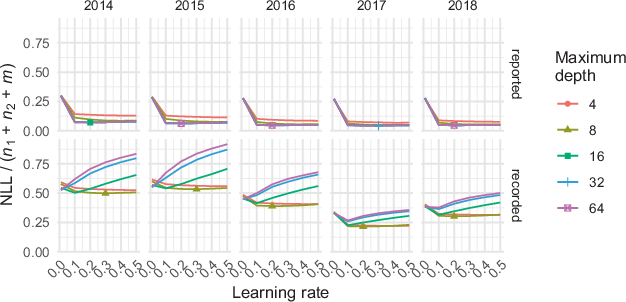
Per year and target variable, the combination of two hyperparameters in the gradient boosting model—learning rate and maximum tree depth—was optimized using K-fold cross-validation. The non-test set was split into

$K=5$

folds of equal size, again stratified by year,

${\delta }_{ij}^{\text{svy}}$

and

${\delta }_{ij}^{\text{sen}}$

. K − 1 = 4 folds were used to train a model with a hyperparameter combination, using a maximum of 100 boosting iterations. Its performance was tested on the remaining fold. This was repeated for each hyperparameter combination and fold. The results were averaged across folds (Figs. 4 and 5). The combination with the lowest NLL was chosen to retrain the model on the entire non-test set, and final performance was measured on the test set.

Fig. 4 Hyperparameter tuning of XGB for binary target variables ${\delta }_{ij}^{\text{svy}}\mid {\delta }_{ij}^{\text{sen}}=1$ (top row) and ${\delta }_{ij}^{\text{sen}}\mid {\delta }_{ij}^{\text{svy}}=1$ (bottom row), per year (columns). Effect of learning rate and maximum depth on logistic negative log likelihood (averaged across K validation sets). Points indicate optimal hyperparameter combination per year

Fig. 5 Hyperparameter tuning of XGB for count target variable y_h, per year (columns). Effect of learning rate and maximum depth on Poisson negative log likelihood (averaged across K validation sets). Points indicate optimal hyperparameter combination per year

4.5 Model performance

) (see Fig. 3). Nevertheless, the balanced accuracy will be 0.5 when flipping a coin or randomly guessing the positive class with its prevalence.

For the count target variable y_h, model performance was measured by the relative root mean squared error (RRMSE):

where

is the number of strata for which the counts y_h are known.

4.6 Variance estimation

Bootstrap methods may be used to obtain variance estimates for both parametric and non-parametric models. For comparability, non-parametric bootstrapping was performed for all estimators discussed in this section. Following Särndal, Swensson, and Wretman (1992, Sect. 11.6), an artificial population of license plate-week combinations was created from the response. Each license plate-week combination was replicated [Rw_i] times, where

was chosen to round non-integer weights to the nearest tenth.

denotes rounding of x using ceiling with probability

and floor with probability

, where d is the second decimal of w_i.

From this artificial population,

bootstrap samples each of size r were drawn with replacement, proportional to size, i.e., with inclusion probabilities

. The number of bootstrap samples is sufficient as the estimates converged around 100 (not shown). Each bootstrap sample of r vehicle-week combinations was expanded by linking the days of the assigned week, survey and sensor indicators

and

, weight w_i, features on vehicles, owners and the number of working sensors, and the test set indicator. Previously selected models were retrained on the training set of each bootstrap sample, using the previously determined optimal hyperparameter combination in case of XGB, and applied to the test set of each bootstrap sample to obtain B bootstrap estimates

per estimator. Each distribution of bootstrap estimates was summarized by the relative standard deviation, i.e., coefficient of variation CV:

For a fair comparison,

and

were also based on the test set only and therefore divided by fraction f.

5 Results

5.1 Model performance on test set

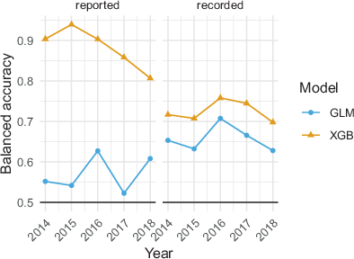
The XGB predictions are of better quality than the GLM predictions, for both the survey indicator (reported) and the sensor indicator (recorded), in all years (Fig. 6). In some years, the GLM models for the survey indicator perform in some years only slightly better than random guessing. The GLM models predict the sensor observations better than the survey observations. Class imbalance is generally stronger in the survey target variable (with a prevalence of about 93%) than in the sensor target variable (with a prevalence of about 22% across years). However, the prevalence in the sensor target variable was only 7% in 2017 (see Fig. 3) without an apparent effect on balanced accuracy. In addition, the XGB models perform better on the survey indicator than on the sensor indicator. Class imbalance is therefore not a likely explanation. The decreasing number of working sensors (see Fig. 2) also does not have an apparent effect on model performance: the year with the least number of working sensors (2017) does not stand out. Other performance metrics, such as the Matthews correlation coefficient or F1 of the positive and negative class show qualitatively similar results (not shown).

Fig. 6 Comparison of model performance between logistic regression (GLM) and gradient boosting (XGB) for binary target variables ${\delta }_{ij}^{\text{svy}}\mid {\delta }_{ij}^{\text{sen}}=1$ (reported) and ${\delta }_{ij}^{\text{sen}}\mid {\delta }_{ij}^{\mathrm{svy}}=1$ (recorded). Performance is measured by balanced accuracy on the test set

The XGB predictions for the counts y_h are also of better quality than the GLM predictions in all years (Fig. 7). The RRMSE is almost halved. In addition, the RRMSE increases over time for GLM—presumably due to the decreased sensor quality (see Fig. 2)—but is fairly constant over time for XGB. The RRMSE is generally large because the mean count in the denominator is small due to the extensive stratification

thousand ).

Fig. 7 Comparison of model performance between Poisson regression (GLM) and gradient boosting (XGB) for count target variable y_h. Performance is measured by $\text{RRMSE}\left({\hat{y}}_h\right)$ on the test set

5.2 Point estimates

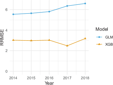
Fig. 8 shows the survey and CRC point estimates by estimator and year. The Huggins and log-linear estimates are compared with two baselines: the single-source weighted survey estimate (solid black line) and the Lincoln-Peterson estimate, a CRC estimate that ignores auxiliary information (dashed black line). The SVY and LP estimates are reasonably constant over time. The same holds for the Huggins and all GLM-based CRC estimates, which are similar to the LP estimates. The combination of LL estimator and XGB model yields point estimates similar to the LP, HUG and LL‑GLM models for the first three years. A large increase in the point estimates, however, can be observed in 2017 and 2018. This is more likely to be caused by a lower number of working sensors than a sudden increase in underreporting. Since this effect is apparent in both LLrepl and LLsupp, the increase is caused by the prediction of the unobserved cell counts (see Eqs. 4 and 5). A prediction as low as 1 for unobserved cells—not included in the RRMSE—can already result in

thousand extra vehicle days (see Table 1). Note that the survey estimate is always lower than any of the CRC estimates (see Sect. 5.4).

Fig. 8 Estimated number of vehicle days $\hat{D}$ by estimator and year. The solid black line is the survey estimate ${\hat{D}}^{\mathrm{SVY}}$ and the dashed black line is the Lincoln-Peterson estimate ${\hat{D}}^{LP}$

5.3 Variance estimates

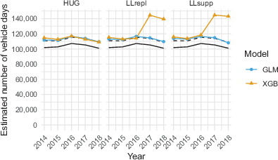
Fig. 9 shows the bootstrapped CVs of the estimated number of vehicle days

by estimator and year. Overall, the CVs can be considered small with errors up to 4%. The CVs of the survey estimates are reasonably constant since the sample size and response rates are fairly stable (see Fig. 1). The CVs of the LP estimates are slightly higher, which is expected since linking the sensor data introduces more uncertainty that is ignored by the survey estimator. Incorporating auxiliary information into the CRC estimators is expected to reduce the CVs again, which is confirmed by the GLM models. The XGB models, however, paint a complex picture. HUG-XGB increases rather than decreases the CVs. The CVs of the LL-XGB initially follow those of the LL‑GLM but spike in the years with few working sensors (2017 and 2018), despite their higher point estimates in the denominator (see Fig. 8).

Fig. 9 Bootstrapped coefficient of variation of estimated number of vehicle days $\hat{D}$ by estimator and year. The solid black line is the CV of the survey estimate ${\hat{D}}^{\mathrm{SVY}}$ and the dashed black line is the CV of the Lincoln-Peterson estimate ${\hat{D}}^{LP}$

5.4 Measurement error

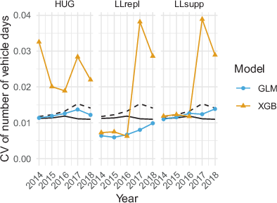
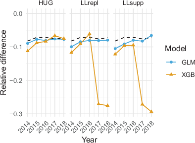
Fig. 10 shows the relative difference of the estimated number of vehicle days

between the survey estimate and a CRC estimate by estimator and year. The relative differences indicate the degree of measurement error in the survey. The survey estimates are 7–8% lower than the LP estimates. The CRC estimators HUG and LL show larger differences than the LP, which does not consider heterogeneity. Hence, including auxiliary information to model heterogeneity increases the relative difference. The XGB-based differences seem less robust than the GLM-based differences, and in 2017 and 2018, unreasonably large differences were found.

Fig. 10 Relative difference between the survey and CRC estimates, $\frac{{\hat{D}}^{\mathrm{SVY}}}{{\hat{D}}^{\mathrm{CRC}}}-1$, by estimator and year. The dashed black line is the annual relative difference between the survey estimate and the Lincoln-Peterson estimate ${\hat{D}}^{LP}$

5.4.1 Discussion

Second, we are not able to assess which of the studied estimators and models has the smallest bias and the correct estimated population variance. We are only able to study which model-estimator combination is the most precise. This problem can be solved with a simulation where the true number of vehicle days is known.

The CRC estimators’ assumptions and required decisions must be mentioned in this regard. The HUG estimator is based on the strong assumption that the conditional likelihood equals the unconditional likelihood (for example, that the probability of being recorded by a sensor given reported used in the survey is the same as the probability of being recorded by a sensor). We consider this a strong and implausible assumption. The LL estimator assumes no interaction between

and

given the auxiliary information. However, the auxiliary information (features) to stratify have to be chosen in advance. Without any theory on which features to select, this decision is data-driven and might result in implausible CRC estimates. A model with too few strata would result in underdispersion and with a too-detailed model, there is the risk of overdispersion. Of course, the choice of features could be optimized, but this has no point without any true value given.

Lastly, we did not correct for days without sensors, but we included the daily number of working sensors in the models. We consider this a minor limitation with little effect on the outcomes.

6 Conclusion

Thereby, it was shown that non-probability data collected, for example, through sensors, cannot be expected to have alltime high quality. Such systems, as used in this paper, need to be maintained; they might break down, resulting in erroneous measurements or record no measurements at all. Accordingly, using such systems as the only data source used to produce official statistics cannot be recommended without hesitation (see for example Klingwort & Burger, 2023). Therefore, using such data to complement and enhance existing and high-quality data sources seems recommended.

Furthermore, this work demonstrated the first application of machine learning in capture-recapture research to estimate survey measurement errors. It was shown that gradient boosting outperformed the traditional generalized linear regression models on the labeled data, but when used in CRC estimators gradient boosting could result in implausible point estimates and high variance.

Acknowledgements

We would like to thank the editor and an anonymous reviewer for their useful comments on an earlier version of this paper.

The views expressed in this paper are those of the authors and not necessarily reflect the policies of Statistics Netherlands.

MW: Software, Validation, Formal analysis, Investigation, Data Curation, Writing—Original Draft, Visualization; JK: Conceptualization, Methodology, Software, Validation, Formal analysis, Investigation, Resources, Data Curation, Writing—Review & Editing, Visualization, Supervision, Project administration; JB: Conceptualization, Methodology, Software, Validation, Formal analysis, Investigation, Data Curation, Writing—Review & Editing, Visualization, Supervision.

See the official home page for more information (https://www.cbs.nl/en-gb/our-services/customised-servicesmicrodata/microdata-conducting-your-own-research). For more information, please contact microdata@cbs.nl.

References

Alho, J. M. (1990). Logistic regression in capture-recapture models. Biometrics, 46(3), 623–635. https://doi.org/10.2307/2532083. a, b

Ashley, D., Richardson, T., & Young, D. (2009). Recent information on the under-reporting of trips in household travel surveys. https://australasiantransportresearchforum.org.au/wp-content/uploads/2022/03/2009_Ashley_Richardson_Young.pdf →

Beaumont, J.-F. (2020). Are probability surveys bound to disappear for the production of official statistics? Survey Methodology, 46(1), 1–28. →

Beck, M., Dumpert, F., & Feuerhake, J. (2018). Machine learning in official statistics. arXiv.. https://doi.org/10.48550/arXiv.1812.10422. →

Biemer, P. P. (2010). Total survey error: design, implementation, and evaluation. Public Opinion Quarterly, 74(5), 817–848. https://doi.org/10.1093/poq/nfq058. →

Bohning, D., Van der Heijden, P., & Bunge, J. (2017). Capture-recapture methods for the social and medical sciences. New York: Taylor & Francis. →

Boulesteix, A.-L., & Schmid, M. (2014). Machine learning versus statistical modeling. Biometrical Journal, 56(4), 588–593. https://doi.org/10.1002/bimj.201300226. →

Braaksma, B., & Zeelenberg, K. (2020). Big data in official statistics. Den Haag, Heerlen, Bonaire: CBS. →

Breiman, L. (2001). Statistical modeling: the two cultures. Statistical Science, 16(3), 199–231. https://doi.org/10.1214/ss/1009213726. →

Carciotto, A., & Signore, M. (2021). Improving relevance: Istat experience on experimental statistics. Statistical Journal of the IAOS, 37(2), 1–9. https://doi.org/10.3233/SJI-200764. →

Centraal Bureau voor de Statistiek (2021). Basisbestanden goederenwegvervoer 2019. Den Haag, Heerlen, Bonaire: CBS. →

Chen, T., & Guestrin, C. (2016). XGBoost: A scalable tree boosting system. In Proceedings of the 22nd acm sigkdd international conference on knowledge discovery and data mining (pp. 785–794). https://doi.org/10.1145/2939672.2939785. a, b

De Broe, S., Struijs, P., Daas, P., van Delden, A., Burger, J., van den Brakel, J., & Ypma, W. (2021). Updating the paradigm of official statistics: New quality criteria for integrating new data and methods in official statistics. Statistical Journal of the IAOS, 37(1), 343–360. https://doi.org/10.3233/SJI-200711. →

Eurostat (2016). Road freight transport methodology: manuals and guidelines. Luxembourg: Publications Office of the European Union. https://ec.europa.eu/eurostat/web/products-manuals-and-guidelines/-/ks-gq-16-005 →

Eurostat (2017). European statistics code of practice for the national statistical authorities and eurostat (eu statistical authority). https://ec.europa.eu/eurostat/documents/4031688/8971242/KS-02-18-142EN-N.pdf/e7f85f07-91db-4312-8118-f729c75878c7 →

Fienberg, S. E. (1972). The multiple recapture census for closed populations and incomplete 2^k contingency tables. Biometrika, 59(3), 591–603. https://doi.org/10.2307/2334810. a, b

Galesic, M., Bruine de Bruin, W., Dalege, J., Feld, S. L., Kreuter, F., Olsson, H., & van der Does, T. (2021). Human social sensing is an untapped resource for computational social science. Nature, 595(7866), 214222. https://doi.org/10.1038/s41586-021-03649-2. →

Grimmer, J., Roberts, M. E., & Stewart, B. (2021). Machine learning for social science: an agnostic approach. Annual Review of Political Science, 24(1), 395–419. https://doi.org/10.1146/annurev-polisci-053119-015921. →

Horvitz, D. G., & Thompson, D. J. (1952). A generalization of sampling without replacement from a finite universe. Journal of the American Statistical Association, 47(260), 663–685. https://doi.org/10.2307/2280784. →

Huggins, R. (1989). On the statistical analysis of capture experiments. Biometrika, 76(1), 133–140. https://doi.org/10.1093/biomet/76.1.133. a, b

James, G., Witten, D., Hastie, T., & Tibshirani, R. (2021). An introduction to statistical learning: With applications in (Second). Springer. →

James, G., Witten, D., Hastie, T., Tibshirani, R., & Taylor, J. (2023). Tree-based methods. In an introduction to statistical learning: with applications in pyth (pp. 331–366). https://doi.org/10.1007/978-3-031-38747-0_8. →

Khodadost, M., Fattahi, A., Nejad, N. H., Shokri, A., Fattahi, H., Sarvi, F., & Mosavi-Jarrahi, A. (2022). Geographic distribution and estimating the childhood cancer incidence in Iran: Three-source capture-recapture analysis on national registries data. Iranian Journal of Public Health, 51(3), 659668. https://doi.org/10.18502/ijph.v51i3.8943. →

Klingwort, J. (2020). Correcting survey measurement error with big data. https://doi.org/10.17185/duepublico/72081. a, b, c

Klingwort, J., & Burger, J. (2023). A framework for population inference: combining machine learning, network analysis, and non-probability road sensor data. Computers, Environment and Urban Systems, 101976, 103–976. https://doi.org/10.1016/j.compenvurbsys.2023.101976. →

Klingwort, J., Buelens, B., & Schnell, R. (2019). Capturerecapture techniques for transport survey estimate adjustment using permanently installed highwaysensors. Social Science Computer Review, 39(4), 527–542. https://doi.org/10.1177/0894439319874684. a, b, c, d, e, f, g, h

Klingwort, J., Burger, J., Buelens, B., & Schnell, R. (2021). Transition from survey to sensor-enhanced official statistics: road freight transport as an example. Statistical Journal of the IAOS, 37(4), 12891299. https://doi.org/10.3233/SJI-210821. a, b, c, d, e, f, g, h

Krishnamurty, P. (2008). Diary. In P. J. Lavrakas (Ed.), Encyclopedia of survey research methods (Vol. 1, pp. 197–199). Thousand Oaks: SAGE. →

Larson, A., Stevens, A., & Wardlaw, G. (1994). Indirect estimates of ‘hidden’ populations: Capturerecapture methods to estimate the numbers of heroin users in the australian capital territory. Social Science & Medicine, 39(6), 823–831. https://doi.org/10.1016/0277-9536(94)90044-2. →

Lincoln, F. C. (1935). The waterfowl flyways of north america. Washington: U.S. Department of Agriculture. a, b

McCrea, R., & Morgan, B. J. T. (2014). Analysis of capture-recapture data. https://doi.org/10.1201/b17222. →

Petersen, C. G. J. (1893). On the biology of our flat-fishes. Kjøbenhaven: The Danish Biological Station. a, b

Puts, M. J. H., & Daas, P. J. H. (2021). Machine learning from the perspective of official statistic. The Survey Statistician, 84, 12–17. →

Rankin, R. W. (2017). EM and component-wise boosting for hidden Markov models: a machine-learning approach to capture-recapture. bioRxiv. https://doi.org/10.1101/052266. →

Richardson, A. J., Ampt, E. S., & Meyburg, A. H. (1996). Nonresponse issues in household travel surveys. In T. N. R. Council (Ed.), Conference proceedings 10: household travel surveys. Washington. (pp. 79–114). →

Särndal, C.-E., Swensson, B., & Wretman, J. (1992). Model-assisted survey sampling. New York: Springer. →

Venables, W. N., & Ripley, B. D. (2002). Modern applied statistics with s (Fourth). New York: Springer. →

Whytock, R. C., Świeżewski, J., Zwerts, J. A., BaraSłupski, T., Pambo, A. F. K., Rogala, M., & Abernethy, K. A. (2021). Robust ecological analysis of camera trap data labelled by a machine learning model. Methods in Ecology and Evolution, 12(6), 1080–1092. https://doi.org/10.1111/2041-210X.13576. →

Yee, T. W., Stoklosa, J., & Huggins, R. M. (2015). The VGAM Package for Capture-Recapture Data Using the Conditional Likelihood. Journal of Statistical Software, 65(5), 1–33. https://doi.org/10.18637/jss.v065.i05. →