Predicting Survey Nonresponse with Registry Data in Sweden between 1993 and 2023: Cohort Replacement or a Deteriorating Survey Climate?
827810.18148/srm/2025.v19i2.8278Predicting Survey Nonresponse with Registry Data in Sweden between 1993 and 2023: Cohort Replacement or a Deteriorating Survey Climate?
https://orcid.org/0000-0003-4096-988XSebastian
Lundmark sebastian.lundmark@som.gu.se University of Gothenburg P.O. 710,
SE 405 30 Gothenburg Sweden
https://orcid.org/0000-0002-1941-5922Kim
Backström kim.backstrom@abo.fi Åbo Akademi University Strandgatan 2 65100 Vasa Finland
247192025European Survey Research Association
Declining response rates have remained a major worry for survey research in the 21st century. In the past decades, it has become harder to convince people to participate in surveys in virtually all Western nations. Worrisome, declining willingness to participate in surveys (i.e., response propensities) may increase the risk of extensive nonresponse bias. Therefore, a better understanding of which factors are associated with survey nonresponse and its impact on nonresponse bias is paramount for any survey researcher interested in accurate statistical inferences. Knowing which factors relate to low response propensities enables appropriate models of nonresponse weights and aids in identifying which groups to tailor efforts for turning nonrespondents into respondents. This manuscript draws on previous theories and research on nonresponse and investigates the risk of nonresponse bias, both cross-sectionally and over time, in two time series cross-sectional studies administered in Sweden (the National SOM Surveys 1993-2023 and the Swedish National Election Study 2022). Capitalizing on available registry data on all sampled persons and their corresponding neighborhood-level contextual data, a meta-analytical analysis of nine years of data collection finds that educational attainment, age, and country of birth are among the strongest predictors of response propensities. However, contextual factors—such as living in socially disadvantaged neighborhoods—also predict willingness to participate in surveys. Furthermore, utilizing the three decades of data, the growing nonresponse could be identified to be wholly attributable to a deteriorating survey climate rather than birth cohort replacement or immigration patterns.
1 Introduction
In the 21st century, survey nonresponse has been rising (Groves, 2006; Kreuter, 2013; de Leeuw et al., 2018, 2020; Luiten et al., 2020; Peytchev, 2013; Leeper, 2019), a trend that shows no signs of stopping (Brick & Williams, 2013). Surveys are used to make inferences and generalizations about a larger population based on a smaller sample rather than studying the entire population (Neyman, 1934). However, a uniformly distributed nonresponse is a prerequisite for accurate inferences and generalizations based on such samples (Groves & Lyberg, 2010). Worryingly, nonresponse has been found to be positively associated with nonresponse bias (i.e., nonresponse that skews the estimates obtained; Cornesse & Bosnjak, 2018), a bias that can become severe if the nonresponse is systematically related to unobserved data (Couper & de Leeuw, 2003; Little & Rubin, 2002). However, some studies find that greater nonresponse might only be weakly related to increased bias (Groves & Peytcheva, 2008), especially when the correlation between nonresponse and the inferential statistic is small (e.g., less than r = 0.07, Hedlin, 2020).
Given that nonresponse is sometimes found to increase bias and sometimes not, further understanding of individuals’ response propensities and the correlates of increasing nonresponse and nonresponse bias is needed. Understanding survey nonresponse and its impact on nonresponse bias enables better statistical modeling and helps survey researchers design interventions that efficiently counteract trends of increasing survey nonresponse. Furthermore, given the decline in response rates in the Western world, understanding whether the response rate decline is due to a changing survey climate (i.e., a general decline in a population’s willingness to participate in surveys) or cohort replacement (e.g., older likely-to-participate cohorts exiting the population and replaced by unlikely-to-participate younger cohorts) will better prepare survey researchers to combat nonresponse in the coming decades.
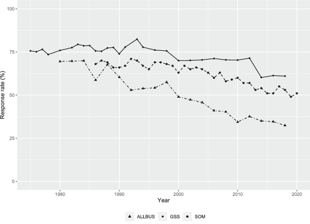
This study extends previous research on nonresponse, the risk of nonresponse bias, and the survey climate by predicting nonresponse with individual and contextual registry data from two time series cross-sectional studies administered to the Swedish population. Assessing decreasing response rates, risk of nonresponse bias, and the survey climate in Sweden serves as a typical case for studying survey nonresponse in Western liberal democracies (Yin, 2003, p. 41) as response rates in the Swedish context have followed the same trend of declining response rates as found in major survey projects in other countries (see Fig. 1). The response rates in the Swedish studies serve as a middle-ground between the high response rate reported in, for example, the American General Social Survey (GSS) and the slightly lower rates reported in the German Social Survey (ALLBUS). Focusing on this middle ground of response rate, while capitalizing on the reliable registry data existent in Sweden, theories on response propensities should be likely to be accurately assessed and generalizable to other Western liberal democracies.


Fig. 1 Response rates reported in GSS (U.S.), ALLBUS (Germany), and the SOM Institute (Sweden)For compiled response rates, see GSS (2023), Schwemmer (2022), and Bergquist et al. (2023). Response rates for the GSS and ALLBUS surveys correspond to RR5 (AAPOR, 2023), according to Gummer (2019). The SOM survey response rates correspond to RR6 (AAPOR, 2023).
Lastly, using the complete records of several demographic characteristics across all sampled persons in the Swedish data, the effect a predictor had on the response propensities could be controlled for the impact of several other predictors. Compared to many other studies on response propensities (e.g., Boyle et al., 2021; Cavari & Freedman, 2022; Keeter et al., 2017), the data presented in this manuscript, therefore, allowed for a more accurate exploration of the impact that demographic factors had on response propensities. The cross-sectional surveys analyzed were collected within the Society, Opinion, and Media Surveys (the SOM Surveys) between 1993 and 2023 (SOM Institute, 2024) and in the Swedish National Election Study (SNES) for the 2022 parliamentary election (SNES, 2023). Benefiting from the long time series and available registry data in the SOM Surveys, an assessment of a deteriorating survey climate and cohort replacement as causes of increasing nonresponse and bias could be estimated for a wider range of demographic characteristics (i.e., immigrant and birth cohorts) than before (e.g., Gummer, 2019). Assessing cohort replacement’s impact on response propensities should allow for more efficient future responsive and adaptive survey designs (i.e., identifying whether surveys should be adapted for specific cohorts of respondents or a changing survey climate).
The manuscript is outlined as follows: First, different theories explaining nonresponse and the survey climate, predictors of nonresponse identified in previous research, and how the risk of nonresponse bias and cohort change relate to nonresponse are reviewed. Second, data and measurements, description of the analytical plan, including meta-analytical regressions, R indicators, dissimilarity indices, and decompositions of change are discussed. Lastly, the results of the analyses and their implications for survey methodology and future research are presented.
2 Nonresponse in Surveys: Theories and Survey Climate
Several theories have outlined what causes a sampled person to exert the effort to participate in surveys (Dillman, 2020), of which social exchange theory (SET) and leverage-salience theory (LST) have dominated the literature. SET centers around the view that the perceived benefits (e.g., incentives, answer uniqueness), perceived costs (e.g., length, complexity), and trust that the benefits will outweigh the costs determine survey cooperation (Dillman et al., 2014, p. 25). Similarly, LST holds three main components: leverage, salience, and valence (Groves et al., 2000). Leverage relates to how vital an individual perceives a survey attribute. Salience relates to whether the individual notices those attributes or not. Valence determines whether the survey attribute’s leverage and salience nudge the individual towards survey cooperation or nonresponse. However, the same survey attribute may result in several different outcomes on survey cooperation at the individual level, creating a need to study response propensities further to counteract survey nonresponse better.
SET and LST are often used to understand how to convert nonrespondents to respondents, for example, using Responsive and Adaptive Survey Designs (RASD) by tailoring survey requests based on individual or contextual characteristics (Schouten et al., 2017; Tourangeau et al., 2017). But to apply RASD, one first needs to understand whether declining response rates are due to cohort replacement or a worsening survey climate. That is, suppose that nonresponse has increased even though the protocol of a repeated cross-sectional survey (e.g., sampling method or the number of reminders) has been kept identical over time. In such a case, a deteriorating survey climate could explain the declining response rates. However, the decline could also be caused by the composition of the population (e.g., high response propensity cohorts being exchanged with low response propensity ones). In the context of SET, a deteriorating survey climate could lead to sample persons no longer trusting that the benefits outweigh the costs of participating in the surveys, or in the context of LST, general interest in the survey topic might not effectively leverage survey participation as a new cohort enters the population (e.g., new birth cohorts or immigrants being disinterested in the topic). Predicting response propensities helps improve nonresponse adjustments and RASD, offering insights into how nonresponse may evolve, given the sharp decline in response rates since the 1990s (Brick & Williams, 2013; Gummer, 2019).
3 Predictors of Nonresponse in Surveys
Several explanations for the global increase in survey nonresponse has been proposed based on the theories such as the SET and LST. These can be divided into nonresponse predictors at the individual and contextual levels. At the individual level, factors such as educational attainment, age, migrant status, sex, income, welfare status, illiteracy, and marital status have often been suggested as predictors of nonresponse and to correlate with attitudinal characteristics predictive of nonresponse (Keeter et al., 2006; 2017; Rogelberg & Luong, 1998; Groves & Couper, 1998; Shaghaghi et al., 2011; Bates, 2017; Kreuter et al., 2010). Among these individual factors, educational attainment has been the most prominent (Keeter et al., 2017). Spending less time in the educational system correlated with higher nonresponse (Keeter et al., 2006; Rogelberg & Luong, 1998; van Wees, 2019), and relatedly, illiteracy appears predictive of nonresponse (Shaghaghi et al., 2011). Additionally, suffering from economic hardship, such as having a lower household income or being a benefit recipient, predicted nonresponse (Abraham et al., 2006; Bates & Mulry, 2011; Brick & Williams, 2013; Groves & Couper, 1998; Shaghaghi et al., 2011). Furthermore, income level tends to correlate with educational attainment (Breen & Chung, 2015; Naito & Nishida, 2017), adding a possible double curse of low income and low educational attainment on decreasing response propensities.
Similarly, less political interest and political knowledge predicted greater nonresponse, even in surveys with only a partial focus on politics (Keeter et al., 2006; Keeter et al., 2017). Furthermore, as with income, educational attainment appears to be a strong predictor of political interest and political knowledge (Coffé & Michels, 2014; Rapeli, 2022), indicating yet another reason for education to be one of the most important factors for response propensities.
Generally, younger age has been found predictive of greater nonresponse (van Wees et al., 2019; Eisele, 2017). Bates (2017) found that young adults were harder to reach than other groups due to moving more frequently and being more likely to rent their homes. However, the choice of survey mode may play a part here. For example, younger people seem to prefer online survey modes over other modes (Bates, 2017; Hartman & McCambridge, 2011). Furthermore, greater nonresponse among younger people correlated with higher nonresponse from individuals suffering from economic hardships (Abraham et al., 2006; Bates & Mulry, 2011; Brick & Williams, 2013). In addition, younger people have been found to be less politically interested and knowledgeable than others (García-Albacete, 2014; Rapeli, 2022), potentially increasing the risk of nonresponse.
Furthermore, being foreign-born (Bates, 2017; Eisele, 2017; Shaghaghi et al., 2011; van Wees et al., 2019) or a non-citizen (Kreuter et al., 2010) have predicted nonresponse. For example, Bates and Mulry (2011) found that a greater nonresponse among immigrants was linked to language barriers, unfamiliarity with the survey organization, and fearing the organization behind the survey. These findings align with other findings indicating that lower social and political trust was linked to greater nonresponse (Brick & Williams, 2013; Couper & de Leeuw, 2003; Shaghaghi et al., 2011). Inferred from other research topics, immigrants should also be expected to be less politically interested and knowledgeable than natives (Fennema & Tillie, 2001; González-Ferrer, 2011).
Lastly, males have been found to be slightly less likely than females to complete questionnaires (van Loon et al., 2003; Rogelberg & Luong, 1998), as were widowed people, people living in childless and single-person households (Abraham et al., 2006; Bergstrand et al., 1983; Groves, 2006), and those socially excluded (Keeter et al., 2017). Forms of social exclusion have, in turn, been associated with lower social trust (Twenge et al., 2007), and low-trusting individuals can be expected to be more critical toward the survey organization, which also have been found to correlate with nonresponse (Keeter et al., 2006).
However, research have identified that factors at the contextual level may be predictive of nonresponse. Areas where a greater share of accommodations were rentals, the income level was lower, a greater share of the population received benefits, unemployment was high, or the education level was low were all found to predict greater nonresponse (Bates & Mulry, 2011; Brick & Williams, 2013). In contrast, Brick and Williams (2013) found that a higher crime rate was associated with a greater likelihood of completing surveys. Nevertheless, Brick and Williams (2013) underlined that they studied crime rates at the national level over time, allowing for the possibility that local variations in crime rates may have gone unnoticed.
In a Swedish context, the above-listed contextual factors coincide with areas the Swedish Police have identified as socially disadvantaged. These disadvantaged areas tended to have a greater proportion of immigrants, people in economic hardship, lower trust in authorities, and a greater proportion of crimes (especially organized crime) than other areas in Sweden (Swedish Police, 2015). Such contextual data may, therefore, be important to leverage when designing RASDs and following SET and LST to improve response rates, especially when focusing on hard-to-reach populations to decrease the risk of nonresponse bias.
4 Dissimilarity, Nonresponse Bias, and Cohort Replacement
Whereas nonresponse rates have increased in Western societies (Brick & Williams, 2013), it is less clear whether nonresponse bias has followed that trend (Curtin et al., 2000; Groves & Peytcheva, 2008; Keeter et al., 2000; Stoop, 2005). Cornesse and Bosnjak (2018) studied data from 69 published articles and found a positive association between nonresponse and nonresponse bias. On the other hand, Groves and Peytcheva (2008) found no substantive relationship between response rates and the amount of nonresponse bias when studying 59 other studies. Similarly, through simulations, Hedlin (2020) found that nonresponse bias seemed to increase only when response rates fell below 30%. Above this “safe area,” nonresponse appeared to only marginally bias estimates (Hedlin, 2020). Given these inconsistent findings, investigating the relationship between predicted individual response propensities, nonresponse bias, and response rates may provide insights for survey methodologists. However, it is important to note that nonresponse bias is estimate-specific (Bethlehem, 2002). That is, the degree of bias changes based on the variables estimated. So, whereas the previous chapter showed that demographic aspects may be important predictors of nonresponse, there is no guarantee that these predictors lead to bias in specific estimates. Therefore, it is more accurate to use the term “risk of nonresponse bias” when discussing bias not specific to a certain estimate and we adopt such nomenclature here.
The relationship between declining response rates and nonresponse bias can also be studied by modeling whether dissimilarities between respondents and sampled persons (or the population of which statistical inferences are to be made) have increased over time. Modeling changes in dissimilarity between respondents and nonrespondents over time enables the assessment of whether these changes are due to likely-to-participate cohorts exiting the population and replaced with unlikely-to-participate cohorts (cohort replacement) or whether the changes stem from other sources (e.g., a deteriorating survey climate) (Brick & Williams, 2013; Gummer, 2019). In such models, a cohort comprises individuals who share a characteristic or experience within a period; for example, people born during a specific period (i.e., birth cohorts). When studying birth cohorts’ response propensities, it is important to consider the interplay of age, period, and cohort effects (Yang & Land, 2013). Age effects result from individuals aging, period effects result from external factors at a point in time (e.g., a societal crisis), and cohort effects are the results of the unique experiences of a group.
When analyzing cross-sectional data from a single time point, age and cohort effects are confounded. However, this confound can be counterbalanced by using repeated cross-sectional data over longer time-periods and by estimating age-period-cohort analyses (Yang & Land, 2013, 16–17). Gummer (2019) assessed cohorts in the ALLBUS and GSS 1980–2012 through such an analysis and found that changes in dissimilarities were most likely due to a deterioration of the survey climate and not cohort replacement.
Assessing how birth cohorts enter and exit a population and how their response propensity change as they age, age-period-cohort analyses can decompose the response propensities in what is attributable to aging in general (age), what is attributable to specific cohorts entering or exiting the population (cohort), and what is attributable to society-wide fluctuations or changes influencing survey participation (period). A society fluctuation may be election years when individuals may be more likely to complete questionnaires (however, assessing period effects is beyond the scope of this manuscript). The three effects (age, period, and cohort effects) are necessarily linearly related to each other but can—through analyses—be separated into individual contributions to changes in response propensities.
The literature review suggested that older age may lead to higher response propensities. This means that individuals in a cohort may become more likely to complete questionnaires as they age. A potential explanation for decreasing response rates could be that likely-to-respond older birth cohorts exit the population (e.g., have died or moved) and are replaced by more reluctant-to-respond younger birth cohorts. This would show up in an age-cohort-period analysis as a between cohort change (BCC). If sampled persons, in general, change their perceptions of the benefits and costs of survey participation (which the SET posits predict response propensity) or change their perceptions of what survey attributes are salient and hold leverage (which LST posits predict response propensity), one would instead find a within cohort change (WCC) as the primary explanation for declining response rates.
This age-period-cohort logic can be applied to other cohorts as well. For example, cohorts of immigrants, where unlikely-to-participate immigrants from some geographical areas replace likely-to-participate immigrants from other geographical areas (in a migration-period-cohort analysis). Such a cohort replacement may be especially likely to affect response propensities in countries like Sweden, where the share of the foreign-born population increased rapidly in the past two decades, from 11% of the population being foreign-born in 2000 to 21% foreign-born in 2023 (Statistics Sweden, 2024).
Studying nonresponse predictors and cohorts allows us to decipher whether the increase in nonresponse (and the risk of nonresponse bias due to heterogeneous response propensities and low response rate) is due to a deteriorating survey climate or cohort replacement.
5 Research Questions
Based on our overarching purpose of mapping what predicts response propensities and assessing the risk of nonresponse bias in surveys to improve future studies’ ability to employ RASD approaches according to, for example SET and LST, four research questions were explored:
What individual and contextual factors predict response propensities?
Have the predictors of response propensities changed over time?
Has the risk of nonresponse bias increased over time?
Are changes in the risk of nonresponse bias due to cohort replacement or a changing survey climate?
6 Methods and Materials
6.1 Sample 1
Sample 1 was collected by the SOM Institute, University of Gothenburg, through annually administered surveys between 1993 and 2023 (SOM Institute, 2024). The SOM Institute has since 1986 administered omnibus-style self-administered paper-and-pencil questionnaires to a simple random sample of people living in Sweden. Since 2012, respondents were offered to complete the questionnaire both online and on paper and since 2017 also offered a conditional incentive in the form of a lottery scratcher ticket. The survey questions covered public opinion, attitudes, and behavior toward news media, politics, and society. All survey questions were created in collaboration with researchers and several Swedish government agencies, and the SOM Institute developed all questions administered. Each questionnaire started with questions on news media consumption and then covered the topics of the collaborating researchers and government agencies.
Each annual sample was a simple random sample of the Swedish population drawn from the Swedish Tax Authority registry. Any person registered as living in Sweden between the ages 16 and 85 could be sampled with the exclusion of individuals with classified registration information (e.g., part of witness protection programs). Institutionalized individuals (e.g., in prison or similar) could be sampled. Between 2021 and 2023, the sample was extended to include individuals aged 86–90 years old, but to facilitate comparison, respondents older than 85 were excluded from our analyses. For the response propensity analyses, only data from 2015–2023 was used because registry data for socially disadvantaged areas and country of birth could not be appended to the other years.
6.2 Sample 2
Sample 2 was collected by the Swedish National Election Studies (SNES), University of Gothenburg, and administered before and after the Swedish parliamentary election 2022 (SNES, 2023). Since 1956, SNES have administered face-to-face questionnaires to random samples of people eligible to vote and registered as living in Sweden. In 2018, SNES completed its conversion from face-to-face (that had started in 2014) to self-administered online and paper-and-pencil questionnaires. To make Samples 1 and 2 comparable (keeping survey mode identical), only SNES data from 2022 was included in the analyses (2018 SNES data did not include accurate registry data due to legal obstacles).
The SNES 2022 included three different versions of the questionnaire of which Version 1 was administered before the election (AAPOR RR1 = 35%), and Version 2 after the election (AAPOR RR1 = 34%), and were administered by Statistics Sweden (SCB). The simple random samples for Versions 1 and 2 were drawn prior to the election 2018 and were invited to complete questionnaires in both the election 2018 and 2022 as part of a panel study. Version 3 (AAPOR RR1 = 45%) was a simple random sample drawn prior to the 2022 election, administered after the election, and administered by the SOM Institute. Sampled persons in Version 3 were offered a lottery scratcher ticket conditional incentive, whereas no incentives were offered for Versions 1 and 2. Across all three versions, the questions related to political media consumption, political attitudes, and political behavior. All three simple random samples were drawn by Statistics Sweden. Any person eligible to vote in the Swedish national parliamentary election of 2018 (Versions 1 and 2) or 2022 (Version 3) and registered as living in Sweden was allowed to be sampled, with the exclusion of individuals with classified registration information (e.g., part of witness protection programs). Institutionalized individuals (e.g., in prison or similar) could be sampled. To be eligible to vote in the national parliamentary election, a person had to be a Swedish citizen aged 18 or older on the day of the election.
6.3 Measurements
6.3.1 Individual Factors
A variable called responded was coded 1 for sampled persons who answered more than 80% of the eligible questions and 0 for sampled persons who answered 80% or fewer of the eligible questions (following AAPOR, 2023, Response Rate 1, RR1).
Sampled persons’ legal sex was extracted from the Swedish Tax Authority registry, and females were coded 1 and males 0. A midwife registered the sex of any newborns in Sweden, and the Swedish Migration Agency recorded the sex of anyone seeking residency in Sweden. Individuals could change their registered legal sex by submitting a form to the Swedish Tax Authority.
Sampled persons’ years of birth were extracted from the Swedish Tax Authority registry, midwives registered the date and year of birth of any newborns born in Sweden, and the Swedish Migration Agency recorded the age of anyone seeking residency in Sweden. Age was coded to range from 16–85.
Sampled persons’ country of birth was extracted from the Swedish Tax Authority registry, and an individual born in Sweden whose parents were registered as living in Sweden had Sweden reported as their country of birth. The Swedish Migration Agency recorded the country of birth of anyone seeking residency in Sweden. Dummy variables for “born in Sweden,” “born in the Nordics,” “born somewhere in Europe,” and “born somewhere outside of Europe” were created.
Marital status was extracted from the Swedish Tax Authority registry. Individuals who had never been married (i.e., had never submitted a marriage certificate to the Tax Authority) were registered as never married, individuals currently married were registered as married, divorced individuals who were currently not re-married were registered as divorced, and individuals currently not married and whose spouse had died were registered as widow/widower. Dummy categories were created for “never married,” “married,” “divorced,” and “widow/widower.”
Sampled persons’ citizenship was extracted from the Swedish Tax Authority registry. Parents reported any newborn’s citizenship, and the Swedish Tax Authority decided on its eligibility. The Swedish Migration Agency recorded the citizenship of anyone seeking residency in Sweden. Individuals may have more than one citizenship registered. A dummy variable was coded 1 for sample persons who held Swedish citizenship (regardless of whether they also held any other citizenship) and 0 otherwise.
Sampled persons’ level of education was extracted from the Education Registry handled by Statistics Sweden. All schools, universities, colleges, and vocational schools reported which individuals had completed courses to Statistics Sweden. Thus, anyone who had participated in a formal education in Sweden was included in the registry. Foreign-born individuals reported their level of education through a mailed or in-person questionnaire administered by the Swedish Migration Agency or Statistics Sweden. Records of education may, therefore, be less accurate for immigrants. Dummy variables for “Did not finish elementary (less than 9 years),” “Elementary (completed),” “Upper-secondary (started or completed),” “Post-upper-secondary (less than 2 years),” and “Post-upper-secondary (2 years or longer)” were created. Only Sample 2 had access to registry data on education level, in which 1% of the sampled persons had no information on education and were coded as missing in the analyses (60% of those missing were born in Sweden, and 40% were not born in Sweden).
6.3.2 Contextual Factors
Living area was extracted from the Swedish Tax Authority registry. Sampled persons registered as living in the three major Swedish cities (Stockholm, Gothenburg, and Malmö) were coded as 1 and 0 otherwise.
Socially Disadvantaged Areas
In 2015, the Swedish police identified 53 neighborhoods in Sweden as socially disadvantaged, at risk of becoming extremely socially disadvantaged, or extremely socially disadvantaged. To be classified as socially disadvantaged, the area had to have a high crime rate, including widespread organized crime, and be characterized by inhabitants distrusting the police and government authorities. The more organized crime and the less trust in government authorities, the more likely the area was to be identified as “extremely socially disadvantaged.” The areas identified by the police were matched to sample persons’ zip codes for the years 2015–2023 and were coded into four socially disadvantaged dummy categories: “not socially disadvantaged,” “socially disadvantaged,” “at risk of becoming extremely socially disadvantaged,” and “extremely socially disadvantaged.” Zip codes that could be matched to the disadvantaged areas was only recorded for Sample 1.
6.3.3 Analysis Plan
To assess response propensities, the standardized parameters of an OLS regression were estimated for each year that data was collected, predicting whether the respondent completed the questionnaire with the individual and contextual characteristics (see Eq. 1).
A benefit of using registry data over comparing a responding sample to a benchmark sample or population statistics, is that registry data on all sampled persons allow one to assess the effect on response propensities of one predictor controlled for the impact of a multitude of other predictors (e.g., see Gundgaard et al., 2008; Lindström, 1986). Thus, compared to studies assessing response propensities for each characteristic separately (Boyle et al., 2021; Cavari & Freedman, 2022; Keeter et al., 2017), Eq. 1 served as a more valid approach for uncovering which characteristics play a predictive role in response propensities.
To strengthen the analyses, Eq. 1 was estimated for each year separately and then included in a meta-analytical regression model. To make the effect of each predictor comparable and to ensure comparability over the entire time-period, all estimates were standardized, and standardized betas were entered into the meta-analytical regression models. Separate models for each year enabled the estimated parameters to be sensitive to idiosyncratic differences in response propensities stemming from a specific year, which could then be accounted for by the meta-analytical regression. Furthermore, a meta-analytical regression allowed for the assessment of whether the estimated effect size of a predictor significantly varied over the years (for Sample 1) or versions (for Sample 2). Alternative estimation techniques to meta-analytical regression are conceivable. For example, pooling all observations and estimating a multilevel regression model nesting observations within years of data collection would allow for adding predictors of changes to the survey protocols. But exploring such a model rendered identical results to those shown in this manuscript (the alternative model can be found in the SOM, section S2.1.).
Risk of nonresponse bias was assessed by estimating R indicators (Schouten et al., 2009). R indicators are an expression of the standard deviation (SD) of probabilities of responses of units in the population. The R indicators were estimated by first fitting a logistic regression equation of the parameters of sex, age, being foreign-born, marital status, citizenship, education, living in a metropolitan area, and living in a socially disadvantaged area (see Eq. 1), and then estimating Eq. 2 using those parameters (Eq. 2 is equivalent to Eq. 12. in Schouten et al. 2009, and the adjusted R indicators in the R script created by de Heij et al., 2015).
Where ρ is the estimated response probabilities of the n elements. The R indicators yield a value ranging from 0 (complete bias) to 1 (no bias). Complete bias corresponds to the responding sample being orthogonally different from the nonresponding sample on all predictors entered in the model. Conversely, no bias means no difference between the responding and nonresponding samples on the predictors in the model. We see this measure as an indicator of the risks of nonresponse bias. The 95% confidence intervals of the R indicators were estimated following Eq. 24 in Schouten et al. (2009).
Dissimilarity Indices and Decompositions of Change
To assess whether decreasing response propensities were due to cohort replacement or a deteriorating survey climate, corrected dissimilarity indices and decomposition of change were estimated following the method described in Gummer (2019). The dissimilarity index estimates how much the distribution of the responding sample in a demographic variable needs to be changed to resemble the distribution of that variable in the full population. To calculate a dissimilarity index, one first estimates the difference of the relative frequencies r between the responding sample () and the population () within specific cohorts c in the survey i. The formula estimates a cohort-specific dissimilarity () for the survey. The cohort-specific dissimilarities are then added up, yielding an overall dissimilarity index for the ith survey:
For example, the dissimilarity for the birth cohort born 1910–1919 for the 1993 SOM survey was calculated by comparing the relative frequency of respondents () to the population () in 1993, which gave the cohort-specific dissimilarity for that cohort and survey (). The same procedure was then done for all other birth cohorts, and then the cohort-specific dissimilarities were added up to give the dissimilarity index for 1993 ().
However, does not account for differences in cohort size, meaning that small cohorts may greatly impact dissimilarity. Gummer (2019) suggested accounting for this by estimating a corrected dissimilarity index following Eq. 3b:
Here, the corrected dissimilarity index (Di) uses the estimated cohort-specific dissimilarities (dci) and multiplying them by the respective cohort population share (pci) before adding up the total dissimilarity. For example, the 1910–1919 birth cohort comprised only 1% of the population in 2003, whereas the 1960–1969 birth cohort accounted for 18%. Without accounting for differences in the relative size of the cohorts, biases in the two cohorts would have an equal impact on overall dissimilarity.
Furthermore, it is possible to calculate the change in dissimilarity between two time points following Eq. 4a:
Here, the overall change in dissimilarity (ΔD) is calculated by estimating the changes in cohort-specific dissimilarities () and population shares () for time points 1 and 0. For example, we can calculate changes in dissimilarity and population shares for the 1910–1919 birth cohort in dissimilarity and population shares between the 2002 and 1997 SOM surveys. Due to generational replacement, we can reasonably assume that the birth cohort 1910–1919’s population share has decreased. Still, it is unclear whether the cohort’s dissimilarity has increased without looking at data on sample persons.
Finally, the changes in dissimilarity between two time points can be decomposed to identify changes within and between cohorts following Eq. 4b:
These changes in dissimilarity can then be decomposed into within cohort changes (WCC) (e.g., deteriorating survey climate or changes to the survey protocol) and between cohort changes (BCC) (i.e., cohort replacement). A positive WCC indicates that cohorts became more reluctant to complete the questionnaire overall, leading to an increased dissimilarity. A positive BCC indicates that some cohorts with a higher response propensity left the population (e.g., older birth cohorts), while cohorts with a lower response propensity remained or joined the population (e.g., younger birth cohorts), increasing dissimilarity. The total change in dissimilarity is the sum of WCC and BCC. It is important to note that WCC and BCC can counteract each other; a negative WCC may balance out a positive BCC and vice versa. See the online appendix in Gummer (2019) for a more detailed discussion of the formulas and a practical example of how to conduct the calculations.
6.4 Identified Differences and Justification of Sample 1 and 2
Educational level was not recorded in Sample 1 and was not included in models fitted to the data for Sample 1. Similarly, Sample 2 only included Swedish citizens and did not record zip codes, so citizenship and socially disadvantaged areas were not included in models fitted to Sample 2. Lastly, only the last parliamentary election was included in the analyses of Sample 2, rendering a corrected dissimilarity index impossible to estimate. Sample 2, albeit restricted to a single time-point, complemented Sample 1 by adding the predictor educational attainment. Thus, Sample 2 served as an extension and robustness test of the results obtained through Sample 1 by assessing whether the identified predictors in the time series of Sample 1 replicated in size and predictive ability of response propensity even when controlling for educational attainment. Using these two samples to identify predictors of response propensities should serve as strong empirical evidence of which demographic factors relate to response propensities despite their independent limitations.
6.5 Transparency and Openness
None of the evaluation criteria, statistical methods, research questions, and coding of measurements were preregistered prior to analyses and should be considered exploratory (Logg & Dorison, 2021). All analysis syntax to reproduce the results can be found at https://osf.io/g3esh/. Data for Sample 1 is available upon request (University of Gothenburg, SOM Institute, 2024), and data for Sample 2 will be made available after the Swedish Parliamentary Election in 2026 (SND, 2024).
7 Results
7.1 Response Propensity
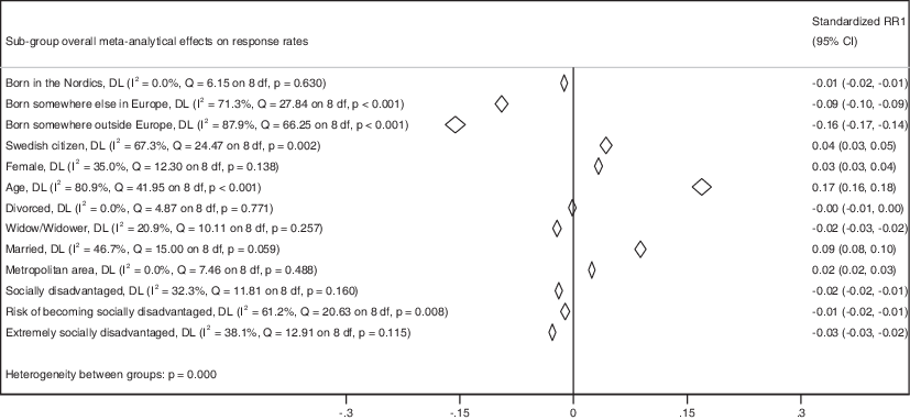
The consistently strongest predictor of response propensity over the nine years (2015–2023) was age (see Fig. 2). The older the sampled persons were, the more likely they were to complete the questionnaire (𝛽pooled = 0.17, p < 0.001, 95% CI[0.16, 0.18]). However, over time, age became a slightly stronger predictor of response propensities (see the SOM, Figure S1) supported by a Cochran’s Q statistic for heterogeneity, indicating a heterogeneous effect size across the data collections (Q(8) = 41.95, p < 0.001) and an I2-statistic that indicated that 81% of the variation of the standardized betas were due to effect heterogeneity.


Fig. 2 Summary predicted response propensities between the years 2015–2023. Diamonds represent the summary meta-analytical regression coefficients obtained from the parameters of nine independent OLS regression models, one model for each year between 2015 and 2023. The widths of the diamonds represent the 95% confidence intervals of the summary meta-analytical regression coefficients. A diamond to the left of the horizontal line over zero meant that the predictor decreased response propensities, and a diamond to the right indicates that the predictor increased response propensities. No sampling weights were applied to any of the data collections. The full meta-analytical regression can be found in SOM, Figure S1.Source: SOM Institute (2024)
The second strongest predictor was the sampled persons country of birth (see Fig. 2). Sampled persons not born in Europe were statistically significantly less likely to complete the questionnaires (𝛽pooled = −0.16, p < 0.001, 95% CI[−0.17, −0.14]) than persons born in Sweden. Similarly, sampled persons born somewhere else in Europe but outside the Nordics were also less likely to complete the questionnaire (𝛽pooled = −0.09, p < 0.001, 95% CI[−0.10, −0.09]), whereas those born in the Nordics but not in Sweden were only slightly less likely to complete the questionnaire (𝛽pooled = −0.01, p < 0.001, 95% CI[−0.02, −0.01]) than persons born in Sweden. Furthermore, the predictive ability of not being born in Sweden on questionnaire completion was heterogeneous over time for those born outside Europe (Q(8) = 66.25, p < 0.001; I2 = 88%) and those born in Europe outside the Nordics (Q(8) = 27.84, p < 0.001; I2 = 71%), but was homogenous for those born in the Nordics (Q(8) = 6.15, p = 0.63; I2 = 0%).
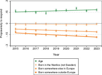
The heterogeneity of the prediction for those born outside of the Nordics stemmed from the fact that sampled persons from those countries became less and less likely to complete the questionnaire compared to persons born in Sweden (see Fig. 3 and SOM, Figure S1). Visualizing these trends for age and migrant status, plotting the standardized regression coefficients in a scatter plot and fitting a regression line, showed the strengthening of the predictive ability of being born outside the Nordics (bborn somewhere outside Europe = −0.007, p < 0.001, 95% CI[−0.01, −0.00]; bborn in Europe, not the Nordics = −0.004, p < 0.001, 95% CI[−0.01, −0.00]) (see Fig. 3). In contrast, age’s predictive ability did not reveal the same statistically significant linear increase in response propensities over the nine cross-sections (bage = 0.003, p < 0.12, 95% CI[−0.00, 0.01]) (see Fig. 3).


Fig. 3 Increased predictive ability of age and country of birth from 2015–2023.Dots represent the standardized OLS regression parameter obtained from nine independent OLS regression models, one model for each year between 2015 and 2023. Bars represent 95% confidence intervals of the predictor. The lines represent an OLS regression fitted line predicting the standardized betas with the year of data collection.Source: SOM Institute (2024)
In addition to age and being an immigrant, several other factors predicted response propensities. Compared to singles, married sampled persons were more likely to complete the questionnaires (𝛽pooled = 0.09, p < 0.001, 95% CI[0.08, 0.10]), widows/widowers were slightly less likely to complete them (𝛽pooled = −0.02, p < 0.001, 95% CI[−0.03, −0.02]), whereas divorcees did not differ compared to single persons in their response propensities (𝛽pooled = −0.00, p = 0.53, 95% CI[−0.01, 0.00]). Also predictive of response propensities, females were more likely than males to complete the questionnaires (𝛽pooled = 0.03, p < 0.001, 95% CI[0.03, 0.04]), as were Swedish citizens (𝛽pooled = 0.04, p < 0.001, 95% CI[0.03, 0.05]) compared to non-citizens.
In addition to individual characteristics, sampled persons who lived in socially disadvantaged areas (𝛽pooled = −0.02, p < 0.001, 95% CI[−0.02, −0.01]), in areas at risk of becoming extremely socially disadvantaged (𝛽pooled = −0.01, p < 0.001, 95% CI[−0.02, −0.01]), and in extremely socially disadvantaged areas (𝛽pooled = −0.03, p < 0.001, 95% CI[−0.03, −0.02]), were slightly less likely to complete the questionnaires than those not living in a disadvantaged area. Controlling for socially disadvantaged areas, sampled persons living in metropolitan areas were more likely to complete the questionnaires (𝛽pooled = 0.02, p < 0.001, 95% CI[0.02, 0.03]) than those living in smaller cities or rural areas.
In line with findings that OLS regressions and nonparametric regressions most often yield identical results even for binary outcomes (Hellevik, 2009; Gomila, 2021), a robustness check estimating the models using probit regression yielded identical conclusions of statistically significant predictors of response propensities and identical relative ranks of the predictors as the OLS-regression results presented here (see SOM, section S2.2.).
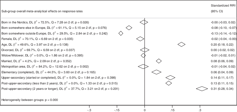
The strongest predictor of response propensities in Sample 2 was educational level (see Fig. 4). Compared to sampled persons who had not completed elementary school (i.e., less than 9 years completed in school), sampled persons who had attended at least 2 years of post-upper secondary education (e.g., at the university or some other higher education) were much more likely to complete the questionnaire (𝛽pooled = 0.32, p < 0.001, 95% CI[0.28, 0.34]). Sampled persons who had completed only some post-upper-secondary (𝛽pooled = 0.13, p < 0.001, 95% CI[0.11, 0.15]), who started or had completed upper-secondary (𝛽pooled = 0.14, p < 0.001, 95% CI[0.11, 0.17]), and who completed elementary school (𝛽pooled = 0.06, p < 0.001, 95% CI[0.04, 0.09]) were also more likely to complete the questionnaire.


Fig. 4 Summary predicted response propensities SNES 2022.Diamonds represent the summary meta-analytical regression coefficients obtained from the parameters of three independent OLS regression models, one model for each version of the questionnaire. The widths of the diamonds represent the 95% confidence intervals of the summary meta-analytical regression coefficients. A diamond to the left of the horizontal line over zero meant that the predictor decreased response propensities, and a diamond to the right indicates that the predictor increased response propensities. No sampling weights were applied to any of the data collections. The full meta-analytical regression can be found in SOM, Figure S2.Source: SNES (2023)
Surprisingly, despite the differences in methodology, response rates, and being able to control for sampled persons’ educational level, the sizes of the predictors of response propensities were remarkably similar in Sample 2 as in Sample 1 (see Fig. 4). In Sample 2, age was again among the strongest predictors, where the older the sampled person was, the more likely they were to complete the questionnaire (𝛽pooled = 0.20, p < 0.001, 95% CI[0.18, 0.22]). Similarly, despite including only Swedish citizens, sampled persons not born in Europe were statistically significantly less likely to complete the questionnaires (𝛽pooled = −0.13, p < 0.001, 95% CI[−0.14, −0.12]) as were those born somewhere else in Europe outside the Nordics (𝛽pooled = −0.08, p < 0.001, 95% CI[−0.10, −0.07]) compared to those born in Sweden. Those born in the Nordics but not in Sweden were not less likely to complete the questionnaire (𝛽pooled = −0.00, p = 0.73, 95% CI[−0.03, 0.02]).
Compared to singles, married sampled persons were more likely to complete the questionnaires (𝛽pooled = 0.08, p < 0.001, 95% CI[0.06, 0.09]), whereas widows/widowers (𝛽pooled = −0.01, p = 0.29, 95% CI[−0.02, 0.01]) and divorcees (𝛽pooled = 0.00, p = 0.96, 95% CI[−0.02, 0.00]) were not more likely than single persons to complete the questionnaire. In contrast to Sample 1, females in Sample 2 were less likely (𝛽pooled = −0.02, p = 0.03, 95% CI[−0.04, −0.00]) than males to complete the questionnaires. Sampled persons living in metropolitan areas were not more likely to complete the questionnaires (𝛽pooled = −0.01, p = 0.61, 95% CI[−0.04, 0.02]) than those living in smaller cities or rural areas.
7.1.1 Nonresponse Bias
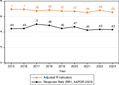
Even though several characteristics predicted response propensities, and some linearly increased in effect size over time, overall bias did not become clearly exacerbated (see Fig. 5). Estimating the adjusted R indicators for each of the nine years, the estimated bias ranged from 0.66 (in 2023) to 0.70 (in 2015), with bias increasing only slightly each year between 2015–2023 (with a fitted OLS line of adjusted R indicator values over years: byear = −0.004, p = 0.02, 95% CI[−0.007, −0.001]). The correlation between the adjusted R indicators and the response rate was moderate (r = 0.26), suggesting that the risk for nonresponse bias might be somewhat related to decreasing response rates.


Fig. 5 Bias (adjusted R indicators) and the response rate for the years 2015–2023.Adjusted R indicators values were based on the discrepancy between respondents and nonrespondents regarding sex, age, being foreign-born, marital status, citizenship, living in a metropolitan area, and living in a socially disadvantaged area, and estimated through logistic regression.Source: SOM Institute (2024)
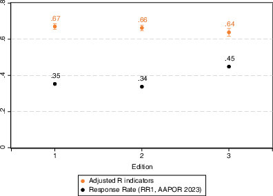
Supporting the results of Sample 1, overall bias did not become exacerbated by a lower response rate in Sample 2 (see Fig. 6). Estimating the adjusted R indicators for each of the survey versions in Sample 2, the estimated bias ranged from 0.64 in the version with the highest response rate to 0.67 in the version with the lowest response rate. Pearson’s r between the adjusted R indicators values and RR1 was r = −0.94, albeit with only 3 observations the coefficient should be interpreted cautiously.


Fig. 6 Bias (adjusted R indicators) and the response rate for the three different editions of the Swedish National Election Study 2022.Adjusted R indicator values were based on the discrepancy between respondents and nonrespondents regarding sex, age, being foreign-born, marital status, education, and living in a metropolitan area, and estimated through logistic regression.Source: SNES (2023)
7.2 Survey Climate or Cohort Replacement?
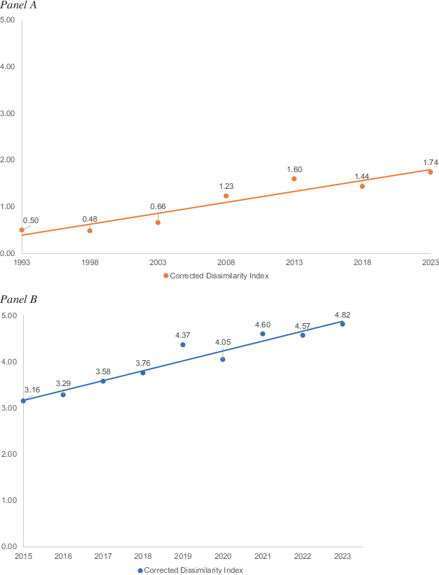
Since 1993, the dissimilarity between birth cohorts steadily increased, starting at D1993 = 0.50 to more than triple the amount in the year 2023 at D2023 = 1.74 (byear = 0.05, p < 0.01, 95% CI[0.03, 0.07]), (see Fig. 7, Panel A). Similarly, assessing the years of data where the country of birth of the sampled persons was available (2015–2023), the dissimilarity between those foreign-born or born in Sweden increased statistically significantly linearly over the entire period starting at D2015 = 3.16 in 2015 to D2023 = 4.82 in 2023 (byear = 0.22, p < 0.001, 95% CI[0.16, 0.27]).


Fig. 7 Corrected dissimilarity index for birth cohorts (Panel A, 5‑year intervals) or being foreign-born or not (Panel B, 1‑year intervals) between 1993–2023.The corrected dissimilarity index was estimated by comparing respondents (RR1) to the full population.Source: SOM Institute (2024).
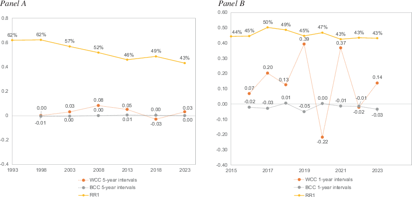
Decomposing these increased dissimilarities into within cohort and between cohort changes, the results highly favored that changing survey climate was the leading cause for the increased dissimilarity rather than less-likely-to-respond cohorts replacing more-likely-to-respond cohorts. That is, as a birth cohort aged (e.g., those born between 1970–1979 going from their mid-thirties in 2008 to their mid-forties in 2018), their willingness to participate increased at a similar pace as what the pace of increased willingness was for other generations going from their forties to their fifties (e.g., as when those born between 1960–1969 went from their forties to fifties). Meanwhile, the deteriorating survey climate made all birth cohorts less willing to participate in surveys. The deterioration of the survey climate over each five-year interval between 1993 and 2023 showed that the survey climate became worse between 1998 and 2013 (WCC2003–1998 = 0.03; WCC2008–2003 = 0.08; WCC2013–2008 = 0.05), while the dissimilarity between cohorts remained completely stable (BCC2003–1998 = −0.00; BCC2008–2003 = 0.00; BCC2013–2008 = 0.01) (see Fig. 8, Panel A). During the same period, the changing survey climate was noticeable, where response rates decreased steadily from 62% (RR1) in 1993 to 43% in 2023, with almost an identical survey protocol across the entire period (only two changes were introduced: paper-and-pencil and web mixed-mode was introduced in 2012, and incentives were introduced in 2017). Between 2013 and 2018, a momentary improved WCC occurred (WCC2018–2013 = −0.03, BCC2018–2013 = 0.00), likely caused by incentives being added to the survey protocol in 2017, leading to an increase in response rates (see Fig. 8, Panel A). However, the incentives caused just a temporary uptick from the overall deteriorating survey climate, in the very next five-year interval, the WCC increased again despite no changes to the survey protocol (WCC2023–2018 = 0.03, BCC2023–2018 = 0.00).


Fig. 8 Decomposition of change and the response rate for birth cohorts (Panel A, five-year intervals) and being foreign-born or not (Panel B, one-year intervals) between 1993–2023.Corrected dissimilarity index estimated by comparing respondents to the full population. WCC means within cohort change, BCC means between cohort change, and RR1 means response rate according to AAPOR, RR1.Source: SOM Institute (2024)
Similarly, over the nine one-year intervals where country of birth was recorded (2015–2023), the survey climate was again found to deteriorate over time (see Fig. 8a, Panel B). In six instances, the within cohort change indicated a deteriorating survey climate (WCC2016–2015 = 0.07; WCC2017–2016 = 0.20; WCC2018–2017 = 0.13; WCC2019–2018 = 0.39; WCC2021–2020 = 0.37; WCC2023–2022 = 0.14), whereas the immigrant cohort replacement had only a little positive impact on the decreasing bias (BCC2016–2015 = −0.02; BCC2017–2016 = −0.03; BCC2018–2017 = 0.01; BCC2019–2018 = −0.05; BCC2021–2020 = −0.01; BCC2023–2022 = −0.03) despite the Swedish population going from 17.02–21% foreign-born in those nine years. The outlying period occurred between 2020 and 2019, where the survey climate temporarily appeared to improve since no changes were made to the survey protocol between those years (WCC2020–2019 = −0.22, BCC2020–2019 = 0.00). In contrast to the effect that adding incentives to the protocol had on the birth cohort analyses, adding incentives did not appear to have the same impact on WCC when analyzing birth country cohorts (where we expected a negative WCC, we saw the same positive WCC2017–2016 = 0.20 as the years prior to the changed survey protocol) (see Fig. 8).
8 Conclusions
The exploration in the present manuscript confirmed previous research findings indicating that educational attainment, age, and country of birth are strong predictors of response propensities. However, unlike most previous studies, this confirmation was obtained even though the impact of each indicator could be controlled for the impact of other indicators such as marital status, area of living, citizenship, and sex of the sampled persons. Diversifying efforts to convert nonrespondents to respondents can be an efficient way to combat declining response rates (Peytchev et al., 2022). When analyzing response propensities of different groups while simultaneously controlling for each contributing factor, the results of the present manuscript aid future survey researchers in identifying where the most urgent efforts to combat nonresponse should be invested. We argue that such efforts should be directed toward those with less formal education, younger persons, and persons not born in the country being studied. Doing so will likely be an efficient way to offset portions of the decline in response rates and its potential for nonresponse bias.
Furthermore, even though the sampling methods and incentivization of respondents differed between the two samples investigated, our analyses revealed almost identical impact of the predictors on response propensities across both samples. This robustness emboldens us to argue that our results likely translate to other Western countries and perhaps even other survey modes than paper-and-pencil/online questionnaires.
Another finding of relevance in this manuscript was that individual-level registry data appeared superior to contextual data for determining response propensities. Given the findings in previous research on contextual factors’ impact on response propensities, one would expect that socially disadvantaged areas in Sweden would have had a strong effect on response propensities (Bates & Mulry, 2011; Brick & Williams, 2013; Keeter et al., 2006). However, the meta-analysis showed that socially disadvantaged areas had only a minor negative effect on response propensities, with much smaller effects than the individual-level predictors. Our findings underline the unavoidable risk of ecological fallacies when using contextual registry data without individual-level data.
However, while the increasing nonresponse among specific groups poses a great challenge for survey researchers wanting to conduct highly powered sub-group analyses, the analyses also showed that declining response rates in medium response rate environments (i.e., between 30–50% RR1) only moderately correlated with greater nonresponse bias risks in terms of estimated R indicators. This serves as an empirical confirmation of simulated studies that have argued that nonresponse bias should be relatively unaffected by decreasing response rates as long as those response rates exceed 30% (Hedlin, 2020). Thus, it appears that the response rates above 30% may indeed exist within a “safe area” of strong influence on nonresponse bias (at least in terms of bias from educational attainment, age, country of birth, sex, citizenship, marital status, urban/rural living, and living in socially disadvantaged areas).
However, further benefiting from the three-decade-long data analyzed, dissimilarity index analysis revealed that the 20-percentage point drop in response rate between 1993 and 2023 was wholly attributable to a deteriorating survey climate and not due to that likely-to-respond birth cohorts died off and were replaced by unlikely-to-respond younger birth cohorts. These findings align with our meta-analytical regressions results that indicated that higher age predicted responses more strongly, meaning that sampled persons became more likely to respond as they aged. In contrast, all birth cohorts became less likely to respond in general, even though they aged during the three decades of data, leading to an increased dissimilarity. Thus, even though our meta-analyses showed that older people were a lot more likely to complete questionnaires, perhaps due to having a more established position in society and more free time, the dissimilarity indices showed that the survey climate deteriorated for all birth cohorts. That is, even though a specific birth cohort became more likely to complete questionnaires as they grew older, they did so at the same pace as other younger birth cohorts.
Similarly, analyzing the country of birth, the results showed that growing dissimilarity between the responding and nonresponding sample in terms of where they were born was attributable to a deteriorating survey climate rather than due to new and more survey reluctant immigrants (e.g., due to language difficulties) immigrating to Sweden. This may be especially surprising given the large influx of new immigrants after the European refugee crisis in 2015, where the Swedish population grew an entire percentage point in a single month (November 2015). These new immigrants appeared en masse in the samples from 2016 and onwards, and our analyses showed no indication that cohort replacement caused the increased dissimilarity. Still, the sharp increase in dissimilarity over time among immigrants warrants further study.
That the survey climate has deteriorated is, of course, bad news for survey research. Unfortunately, the analyses and data in the present manuscript are not equipped to root out causes of the negative trends in the survey climate other than indicating that cohort replacement is not the likely culprit. We urge future research to focus on uncovering the causes of the deteriorating survey climate and exploring interventions aimed at repairing the damage to the climate that has already happened.
A few caveats to our conclusions are warranted. We have studied nonresponse and the risk of nonresponse bias using rich registry data and have found little support that increasing nonresponse leads to an increased risk of nonresponse bias. However, we only had access to registry data on education for a single time point. Whereas the results from both of our samples supported our conclusions, studies on other samples and survey modes are needed.
Furthermore, whereas most of our analyses used data from the SOM survey, the methodological changes during the study period confounded the effect of the deteriorating survey climate on WCC. For example, the introduction of lottery incentives in 2017 improved WCC, while the introduction of mixed mode in 2012 did not have any such clear impact. Still, whereas we cannot determine the exact impact that these two methodological changes had on WCC, our faith remains in that our results support that the survey climate has worsened, and that cohort replacement (BCC) had a negligible impact on nonresponse.
Finally, our findings do not necessarily eliminate the risk of other types of underlying structural biases between respondents and nonrespondents. Previous studies have shown that many sociodemographic variables are related to vital attitudinal indicators, such as political knowledge, political interest, political trust, and social trust (Coffé & Michels, 2014; Keeter et al., 2006, 2017; Rapeli, 2022). However, since there is no registry data on these variables, we cannot determine whether the increasing nonresponse was uniformly distributed across, for example, different levels of political trust. Other analyses, such as nonresponse follow-up surveys or experimentally studying the effect of trying to leverage the survey protocol to facilitate responses from hard-to-reach groups according to SET and LST should be conducted in the future. Also, following Peytchev and Peytcheva (2007), measurement error should be studied to determine if leveraging the survey protocol to facilitate responses from hard-to-reach respondents instead results in increased measurement error.
However, given the currently deteriorating survey climate, from a survey methodological and democratic perspective, it is important to continue studying changes in response propensities and exploring new interventions on how to increase the willingness to participate in surveys both for surveys in general as well as for the respondents who are less willing to do so.
The authors would like to direct thanks to the kind and helpful people at the Society, Opinion, and Media Institute and the Swedish National Election Studies at the University of Gothenburg, Sweden.
This study was in part funded by the Comparative Research Center Sweden (CORS), grant number 2017-00667_VR, the Swedish Research Council, and in part by the Swedish Research Council grant number 2018-01314. The funders did not have a controlling interest in any aspects of the data collection, analyses, or the decision to publish.
Author Contribution
S. Lundmark: Writing—Original Draft (lead), Writing—Review & Editing (equal), Conceptualization (lead), Formal Analysis (lead), Funding acquisition (lead), Methodology (equal), Project administration (equal), Validation (lead), Visualization (equal). K. Backström: Writing—Original Draft (supportive), Writing—Review & Editing (equal), Conceptualization (supportive), Formal Analysis (supportive), Methodology (equal), Project administration (equal), Validation (supportive), Visualization (equal).
1 Supplementary Information
The supplementary information includes Figures of the full meta-analytical regressions and robustness checks of the analyses.The supplementary information includes Figures of the full meta-analytical regressions and robustness checks of the analyses. The supplementary information includes Figures of the full meta-analytical regressions and robustness checks of the analyses. References
AAPOR (2023). Standard definitions—final dispositions of case codes and outcome rates for surveys. https://aapor.org/wp-content/uploads/2023/05/Standards-Definitions-10th-edition.pdf a, b, c
Abraham, K. G., Maitland, A., & Bianchi, S. M. (2006). Nonresponse in the American time use survey: Who is missing from the data and how much does it matter? Public Opinion Quarterly, 70(5), 676–703. https://doi.org/10.1093/poq/nfl037. a, b, c
Bates, N. (2017). The Morris Hansen lecture: hard-to-survey populations and the U.S. census: making use of social marketing campaigns. Journal of Official Statistics, 33(4), 873–885. https://doi.org/10.1515/jos-2017-0040. a, b, c, d
Bates, N., & Mulry, M. H. (2011). Using a geographic segmentation to understand, predict, and plan for census and survey mail nonresponse. Journal of Official Statistics, 27(4), 601–618. a, b, c, d, e
Bergquist, J., Falk, E., & Weissenbilder, M. (2023). The national SOM survey 2022—a metodological overview. https://www.gu.se/sites/default/files/2023-04/4.%20Metodrapport%20Riks%202022.pdf Den nationella SOM-undersökningen 2022—En metodöversikt. →
Bergstrand, R., Vedin, A., Wilhelmsson, C., & Wilhelmsen, L. (1983). Bias due to non-participation and heterogenous sub-groups in population surveys. Journal of Chronic Diseases, 36(10), 725–728. https://doi.org/10.1016/0021-9681(83)90166-2. →
Bethlehem, J. G. (2002). Weighting nonresponse adjustments based on auxiliary information. In R. M. Groves, D. A. Dillman, J. L. Eltinge & R. J. A. Little (Eds.), Survey nonresponse (pp. 275–288). New York: Wiley. →
Boyle, J., Berman, L., Dayton, J., Iachan, R., Jans, M., & ZuWallack, R. (2021). Physical measures and biomarker collection in health surveys: propensity to participate. Research in Social and Administrative Pharmacy, 17(5), 921–929. https://doi.org/10.1016/j.sapharm.2020.07.025. a, b
Breen, R., & Chung, I. (2015). Income inequality and education. Sociological Science, 2, 454–477. https://doi.org/10.15195/v2.a22. →
Brick, J. M., & Williams, D. (2013). Explaining rising nonresponse rates in cross-sectional surveys. Annals of the American Academy of Political and Social Science, 645(1), 36–59. https://doi.org/10.1177/0002716212456834. ISBN 0002716212456. a, b, c, d, e, f, g, h, i, j, k
Cavari, A., & Freedman, G. (2022). Survey nonresponse and mass polarization: the consequences of declining contact and cooperation rates. American Political Science Review. https://doi.org/10.1017/S0003055422000399. a, b
Coffé, H., & Michels, A. (2014). Education and support for representative, direct and stealth democracy. Electoral Studies, 35, 1–11. https://doi.org/10.1016/j.electstud.2014.03.006. a, b
Cornesse, C., & Bosnjak, M. (2018). Is there an association between survey characteristics and representativeness? A meta-analysis. Survey Research Methods, 12(1), 1–13. https://doi.org/10.18148/srm/2018.v12i1.7205. a, b
Couper, M. P., & De Leeuw, E. D. (2003). Nonresponse in cross-cultural and cross-national surveys. In Cross-cultural survey methods (pp. 157–177). New York: Wiley. a, b
Curtin, R., Presser, S., & Singer, E. (2000). The effects of response rate changes on the index of consumer sentiment. Public Opinion Quarterly, 64(4), 413–428. https://doi.org/10.1086/318638. →
Dillman, D. A. (2020). Towards survey response rate theories that no longer pass each other like strangers in the night. In P. S. Brenner (Ed.), Understanding survey methodology: sociological theory and applications (1st edn., pp. 15–44). https://doi.org/10.1007/978-3-030-47256-6_2. →
Dillman, D. A., Smyth, J. D., & Christian, L. M. (2014). Internet, phone, mail and mixed-mode surveys: the tailored design method (4th edn.). Hoboken: John Wiley & Sons, Inc. →
Eisele, P. (2017). Recruitment to the migration attitudes panel. Recruitment rates and demographic differences. https://www.gu.se/sites/default/files/2020-04/LORE_methodological_note_2017_2.pdf SOM Institute. a, b
Fennema, M., & Tillie, J. (2001). Civic community, political participation and political trust of ethnic groups. Connections, 24(1), 198–217. https://doi.org/10.1007/978-3-322-85129-1_9. →
García-Albacete, G. (2014). Young people’s political participation in western europe: continuity or generational change? (1st edn.). London: Palgrave Macmillan. https://doi.org/10.1057/9781137341310. →
Gomila, R. (2021). Logistic or linear? Estimating causal effects of experimental treatments on binary outcomes using regression analysis. Journal of Experimental Psychology: General, 150(4), 700–709. https://doi.org/10.1037/xge0000920. →
González-Ferrer, A. (2011). The electoral participation of naturalised immigrants in ten European cities. In L. Morales & M. Giugni (Eds.), Social capital, political participation and migration in Europe: Making multicultural democracy work? (pp. 63–86). London: Palgrave Macmillan. →
Groves, R. M. (2006). Nonresponse rates and nonresponse bias in household surveys. Public Opinion Quarterly, 70(5), 646–675. https://doi.org/10.1093/poq/nfl033. a, b
Groves, R. M., & Couper, M. (1998). Nonresponse in household interview surveys. Chichester: Wiley & Sons Ltd. a, b
Groves, R. M., & Lyberg, L. (2010). Total survey error: past, present, and future. Public Opinion Quarterly, 74(5), 849–879. https://doi.org/10.1093/poq/nfq065. →
Groves, R. M., & Peytcheva, E. (2008). The impact of nonresponse rates on nonresponse bias: a meta-analysis. Public Opinion Quarterly, 72(2), 167–189. https://doi.org/10.1093/poq/nfn011. a, b, c
Groves, R. M., Singer, E., & Corning, A. (2000). Leverage-saliency theory of survey participation—description and an illustration. Public Opinion Quarterly, 64, 299–308. →
GSS (2023). GSS frequently asked questions. What were the response rates? When did GSS conduct field works? https://gss.norc.org/Lists/gssFAQs/DispForm.aspx?ID=22 →
Gummer, T. (2019). Assessing trends and decomposing change in nonresponse bias: the case of bias in cohort distributions. Sociological Methods and Research, 48(1), 92–115. https://doi.org/10.1177/0049124117701479. a, b, c, d, e, f, g, h
Gundgaard, J., Ekholm, O., Holme Hansen, E., & Kr Rasmussen, N. (2008). The effect of non-response on estimates of health care utilisation: linking health surveys and registers. European Journal of Public Health, 18(2), 189–194. https://doi.org/10.1093/eurpub/ckm103. →
Hartman, J. L., & McCambridge, J. (2011). Optimizing millennials’ communication styles. Business Communication Quarterly, 74(1), 22–44. https://doi.org/10.1177/1080569910395564. →
Hedlin, D. (2020). Is there a ‘safe area’ where the nonresponse rate has only a modest effect on bias despite non-ignorable nonresponse? International Statistical Review, 88(3), 642–657. https://doi.org/10.1111/insr.12359. a, b, c, d
De Heij, V., Schouten, B., & Shlomo, N. (2015). RISQ manual 2.1 Tools in SAS and R for the computation of R‑indicators, partial R‑indicators and partial coefficients of variation. http://www.cros-portal.eu/sites/default/files/NTTS2013fullPaper_63.pdf →
Hellevik, O. (2009). Linear versus logistic regression when the dependent variable is a dichotomy. Quality and Quantity, 43(1), 59–74. https://doi.org/10.1007/s11135-007-9077-3. →
Keeter, S., Miller, C., Kohut, A., Groves, R. M., & Presser, S. (2000). Consequences of Reducing Nonresponse in a National Telephone Survey. Public Opinion Quarterly, 64(2), 125–148. https://doi.org/10.1086/317759 →
Keeter, S., Kennedy, C., Dimock, M., Best, J., & Craighill, P. (2006). Gauging the impact of growing nonresponse on estimates from a national RDD telephone survey. Public Opinion Quarterly, 70(5), 759–779. https://doi.org/10.1093/poq/nfl035. a, b, c, d, e, f
Keeter, S., Hatley, N., Kennedy, C., & Lau, A. (2017). What low response rates mean for telephone surveys (vol. 15). Washington, D.C.: Pew Research Cente. www.pewresearch.org a, b, c, d, e, f, g
Kreuter, F. (2013). Facing the nonresponse challenge. Annals of the American Academy of Political and Social Science, 645(1), 23–35. https://doi.org/10.1177/0002716212456815. →
Kreuter, F., Müller, G., & Trappmann, M. (2010). Nonresponse and measurement error in employment research: making use of administrative data. Public Opinion Quarterly, 74(5), 880–906. https://doi.org/10.1093/poq/nfq060. a, b
Leeper, T. J. (2019). Where have the respondents gone? Perhaps we ate them all. Public Opinion Quarterly, 83, 280–288. https://doi.org/10.1093/poq/nfz010. →
de Leeuw, E., Hox, J., & Luiten, A. (2018). International Nonresponse trends across countries and years: an analysis of 36 years of labour force survey data survey methods: insights from the field. https://surveyinsights.org/?p=10452 Survey Insights: Methods from the Field. →
de Leeuw, E., Luiten, A., & Stoop, I. (2020). Preface. Journal of Official Statistics, 36(3), 463–468. https://doi.org/10.2478/jos-2020-0024. →
Lindström, H. L. (1986). A general view of nonresponse bias in some sample surveys of the Swedish population. Promemorior från P/STM, 23. ISBN 1988:1-2004:2. →
Little, R. J. A., & Rubin, D. B. (2002). Statistical analysis with missing data (2nd edn.). Hoboken: John Wiley & Sons Inc. https://doi.org/10.2307/1533221. →
Logg, J. M., & Dorison, C. A. (2021). Pre-registration: weighing costs and benefits for researchers. Organizational Behavior and Human Decision Processes, 167, 18–27. https://doi.org/10.1016/j.obhdp.2021.05.006. →
van Loon, A. J., Tijhuis, M., Picavet, S. J., Surtees, P. G., & Ormel, J. (2003). Survey Non-response in the Netherlands: Effects on Prevalence Estimates and Associations. Annals of Epidemiology, 13(2), 105–110.https://doi.org/10.1016/S1047-2797(02)00257-0 →
Luiten, A., Hox, J., & De Leeuw, E. (2020). Survey nonresponse trends and fieldwork effort in the 21st century: results of an international study across countries and surveys. Journal of Official Statistics, 36(3), 469–487. https://doi.org/10.2478/jos-2020-0025. →
Naito, K., & Nishida, K. (2017). Multistage public education, voting, and income distribution. Journal of Economics, 120(1), 65–78. https://doi.org/10.1007/s00712-016-0513-5. →
Neyman, J. (1934). On the two different aspects of the representative method: the method of stratified sampling and the method of purposive selection. Journal of the Royal Statistical Society, 97(4), 558–625. →
Peytchev, A. (2013). Consequences of survey nonresponse. Annals of the American Academy of Political and Social Science, 645(1), 88–111. https://doi.org/10.1177/0002716212461748. →
Peytchev, A., & Peytcheva, E. (2007). Relationship between measurement error and unit nonresponse in household surveys: an approach in the absence of validation data. http://www.asasrms.org/Proceedings/y2007/Files/JSM2007-000404.pdf International Workshop on Household Survey Nonresponse. →
Peytchev, A., Pratt, D., & Duprey, M. (2022). Responsive and adaptive survey design: use of bias propensity during data collection to reduce nonresponse bias. Journal of Survey Statistics and Methodology, 10(1), 131–148. https://doi.org/10.1093/jssam/smaa013. →
Rapeli, L. (2022). What is the best proxy for political knowledge in surveys? PLoS ONE, 17(8), 35994461. https://doi.org/10.1371/journal.pone.0272530. a, b, c
Rogelberg, S. G., & Luong, A. (1998). Nonresponse to mailed surveys: a review and guide. Current Directions in Psychological Science, 7(2), 60–65. https://doi.org/10.1111/1467-8721.ep13175675. a, b, c
Schouten, B., Cobben, F., & Bethlehem, J. (2009). Indicators for the representativeness of survey response. https://www.researchgate.net/publication/267836796 Statistics Canada, Catalogue No, 35(1), 101–113. a, b, c
Schouten, B., Peytchev, A., & Wagner, J. (2017). Adaptive survey design. Abingdon: Taylor & Francis. →
Schwemmer, C. (2022). ALLBUS response rates 1980–2021. https://github.com/cschwem2er/allbus_responserates →
Shaghaghi, A., Bhopal, R. S., & Sheikh, A. (2011). Approaches to recruiting ‘hard-to-reach’ populations into re-search: a review of the literature. Health promotion perspectives, 1(2), 86–94. https://doi.org/10.5681/hpp.2011.009. a, b, c, d, e
SND (2024). Collection Swedish election studies—parliamentary elections. Swedish National Data Service (SND). https://snd.se/en/catalogue/collection/swedish-election-studies—parliamentary-elections. →
SNES. (2023). The Swedish National Election Study Sample 2022. Gothenburg: University of Gothenburg a, b, c
SOM Institute (2024). The national SOM survey cumulative dataset (version 13). Gothenburg: University of Gothenburg. https://doi.org/10.5878/7k7n-yn39. a, b, c, d, e, f, g, h
Statistics Sweden (2024). Foreign born in Sweden. https://www.statistikdatabasen.scb.se/sq/151138 Utrikes födda i Sverige. →
Stoop, I. A. L. (2005). The hunt for the last respondent: nonresponse in sample surveys. https://www.researchgate.net/publication/27686407 Sociaal en Cultureel Planbu. →
Swedish Police (2015). Vulnerable areas—social risks, collective ability and unwanted events. https://polisen.se/siteassets/dokument/ovriga_rapporter/utsatta-omraden-sociala-risker-kollektiv-formaga-och-oonskade-handelser.pdf Utsatta områden—sociala risker, kollektiv förmåga och oönskade händelser. →
Tourangeau, R., Brick, J. M., Lohr, S., & Li, J. (2017). Adaptive and responsive survey designs: a review and assessment. Journal of the Royal Statistical Society. Series A: Statistics in Society, 180(1), 203–223. https://doi.org/10.1111/rssa.12186. →
Twenge, J. M., Ciarocco, N. J., Baumeister, R. F., DeWall, C. N., & Bartels, J. M. (2007). Social exclusion decreases prosocial behavior. Journal of Personality and Social Psychology, 92(1), 56–66. https://doi.org/10.1037/0022-3514.92.1.56. →
van Wees, D. A., den Daas, C., Kretzschmar, M. E. E., & Heijne, J. C. M. (2019). Who drops out and when? Predictors of nonresponse and loss to follow-up in a longitudinal cohort study among STI clinic visitors. PLoS ONE. https://doi.org/10.1371/journal.pone.0218658. a, b, c
Yang, Y., & Land, K. C. (2013). Age-period-cohort analysis. New models, methods, and empirical applications. Boca Raton: CRC Press. a, b
Yin, R. K. (2003). Designing case studies. In Case study research: design and methods (pp. 17–55). Thousand Oaks: SAGE. →
