The Poisson Extension of the Unrelated Question Model: Improving Surveys with Time-Constrained Questions on Sensitive Topics
825210.18148/srm/2024.v18i1.8252The Poisson Extension of the Unrelated Question Model: Improving Surveys with Time-Constrained Questions on Sensitive Topics
Benedikt
Iberl benedikt-jonas.iberl@uni-tuebingen.de
Anesa
Aljovic anesa_aljovic@hotmail.de
Rolf
Ulrich ulrich@uni-tuebingen.de
Fabiola
Reiber reiber@uni-mannheim.de University of Mannheim Mannheim Germany
Eberhard Karls University of Tübingen Tübingen Germany
21182024European Survey Research Association
The Poisson model (Iberl & Ulrich, 2023) is a new survey technique that enables the estimation of how frequently a certain behavior occurs, while employing easy-to-answer yes/no-questions that refer to a specific time frame (e.g., “Did you participate in gambling during the last 12 months?”). In this paper, this model is combined with the unrelated question model (UQM) by Greenberg et al. (1969). The UQM is another survey technique that guarantees complete and objective anonymity to participants in order to achieve more valid survey results when asking sensitive questions (e.g., about drug use). The resulting Poisson extension of the UQM (UQMP) is expected to yield valid estimations for how many participants engage in a researched sensitive behavior, and how regularly they do so. The performance of the UQMP was compared to the performance of the standard Poisson model, employing direct questions, in a survey on drinking and driving. While prevalence estimates differ greatly between the UQMP and the standard Poisson model, the results of both models indicate a high rate of drinking and driving among those German traffic participants who generally engage in this behavior. The different prevalence estimates could be due to the fact that some participants in online studies read instructions superficially, lowering the quality of results; we discuss possible causes for these problems and why the UQMP or similar approaches can be valuable nonetheless.
This work was not presented elsewhere before this publication. The data presented in this work was used in the unpublished master thesis of one of the authors (Aljovic, 2022).
The paper was preregistered via OSF (see https://osf.io/nh6e9). The complete data and analysis code was uploaded at https://osf.io/5pkm4/.
1 Introduction
In survey research, one is often interested in obtaining prevalence estimates describing a certain target behavior. Prevalence estimates can be useful in many politically or socially important fields, such as for the assessment of public opinion or to evaluate the frequency of criminal or risky behavior like drug abuse. Oftentimes, these prevalence estimates are produced by posing yes/no questions that refer to a particular time frame, such as “Did you gamble in the past 12 months” (e.g., Andrie et al., 2019; Atzendorf et al., 2019; Beck et al., 2021; Birkel et al., 2022; Burr et al., 1989; Ferrante et al., 2012; Han et al., 2015; Isolauri & Laippala, 1995; Linton et al., 1998; McCabe et al., 2006; McKetin et al., 2006; Şaşmaz et al., 2014; Sawyer et al., 2018; Virudachalam et al., 2014). In this paper, we will call such questions time-constrained yes/no questions.
However, one might not only be interested in whether the concerning behavior has occurred within a certain time frame, but also how often the behavior is shown. So, besides the information about whether someone was gambling in the last year, a researcher might be interested in the rate of this behavior (i.e., the average frequency of the concerning behavior per time unit). To measure this rate, one could simply ask participants how often they have engaged in the behavior in question within a certain time frame (e.g., “How often did you gamble in the past 12 months?”). This kind of questioning technique is also widely used in prevalence research (e.g., Cullen et al., 2018; Miller et al., 2020; Molinaro et al., 2018; Seitz et al., 2020; Soga et al., 2021). Responding to questions that require more than a simple yes or no answer may present some challenges compared to time-constrained yes/no questions. Answering time-constrained yes/no questions might be quicker and less demanding for participants since they only need to recall one instance of the behavior in question. Although there is no direct research comparing the effort needed to answer time-constrained yes/no questions with those asking about behavior frequency, studies suggest that retrieving multiple memories of events or behavior instances can be more taxing for participants (e.g., Aarts & Dijksterhuis, 1999; Bousfield & Sedgewick, 1944; Echterhoff & Hirst, 2006; Janssen et al., 2011; Schwarz et al., 1991).
In conclusion, these questions share a fundamental weakness: The resulting prevalence estimates are ambiguous and do not yield reliable information about the number of people regularly engaging in the behavior, or trait carriers. For example, in a study on addictive behavior, Andrie et al. (2019) asked students in several European countries whether they gambled in the past 12 months. According to the results, 12.5% of the surveyed participants gambled in the past year (Andrie et al., 2019). Obviously, these results are not conclusive regarding the number of trait carriers, that is, regular gamblers within the student population. Instead, they only yield a punctually relevant prevalence estimation. For instance, there might be gamblers that did not gamble in the past year; so, this past-year prevalence of 12.5% is obviously not the same as the prevalence of gamblers in the underlying population. Assuming otherwise would result in an underestimation of the prevalence one wants to measure. One might try to circumvent this ambiguity by expanding the time frame in the posed question, measuring the lifetime prevalence in the most extreme example. However, with such broad time frames, some respondents who are not gambling on a regular basis, but only did so once or twice a long time ago, might be included in the prevalence estimate, despite one would not describe them as gamblers (Fiedler & Schwarz, 2016). Thus, an inflated estimate would result. Another solution might be to ask the participants directly whether they consider themselves to be gamblers. While this would undoubtedly be the most straight forward approach, self-assessments might yield problematic results as well (e.g., due to social desirability bias).
In the following, we introduce a recently proposed method that can solve both mentioned problems of time-constrained yes/no questions (no information about the rate of the behavior and ambiguity of prevalence estimates due to punctual information) while still using the same kind of questions (Iberl & Ulrich, 2023). Based on a Poisson process, this method might be an efficient solution to these problems compared to the mentioned traditional alternatives.
1.1 The Poisson model: A solution for the problems of time-constrained questions?
This Poisson model (Iberl & Ulrich, 2023) yields prevalence estimates of trait carriers (and, in turn, of non-carriers). Additionally, it becomes possible to estimate the rate of the behavior in question. Nonetheless, nothing changes for the participants — they still get asked simple time-constrained yes/no questions; however, they are split into multiple groups. Between groups, the questions are varied slightly: For each group, the respective question refers to a different time-frame t. Since the Poisson model is based on a Poisson process, it can be used to describe any form of behavior that can be assumed to occur regularly and periodically, for example, driving a car, drinking coffee, or smoking cigarettes.
In Fig. 1, the Poisson model is depicted as a probability tree. This tree shows the probability of answering “yes” or “no” to any question on whether a respondent behaved in a certain way in a specific time frame t. According to the model, the probability of being a carrier is π, with the probability of being a non-carrier being defined by 1−π.

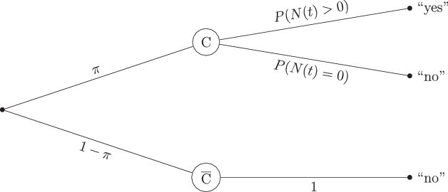
Fig. 1 Probability tree of the Poisson model.The sample is divided into carriers C and non-carriers by the parameter π, describing the probability of a random participant being a carrier of the researched attribute. Non-carriers answer “no” with a probability of 1. Carriers answer “yes” with a probability or “no” with a probability of
Non-carriers, who are represented in the lower branch of the tree, would always answer “no” to a question asking whether they behaved in a certain way (e.g., whether they gambled) in a certain time frame t. The probability of a no-answer would always be 1 for non-carriers, regardless of the time frame, because they do not engage in the behavior in question. For carriers, on the other hand, two answers are possible. One group of carriers could answer “no”, because they did not show the behavior in the time frame t referred to in the question
. The other group of carriers might have engaged in the behavior at least once in the time frame (so
, and would thus answer “yes”.
Since we assume the behavior to be Poisson distributed, N(t) represents a random variable with the rate parameter λ, which denotes the average number of occurrences of the target behavior per time unit. In other words, the reciprocal of λ is the average interoccurrence time. In addition, the probability of k occurrences of the target behavior within the time frame t is given by
1
Thus, the probability of a no-answer is
2
A random participant would answer with “yes” to the time-constrained prevalence question with the probability
3
or
4
Inserting the formula of the Poisson process, one gets the prevalence curve,
5
depicting the prevalence of the behavior as a function of time, with the parameters π and λ determining the asymptote and the slope of the curve, respectively. Fig. 2 shows exemplary prevalence curves and the effects of different parameter values for π and λ.


Fig. 2 Examples of prevalence curves as a function of π and λ with varying values for both parameters
The estimation of the parameters π and λ is enabled by using multiple groups of participants. As mentioned before, the time frame t of the question is varied between groups. For example, one group of participants would be asked if they gambled in a time frame of
week, while another would be asked the same question referring to the time frame of
weeks, and so on. With at least two time frames ti, it is possible to estimate π and λ and thus determine the prevalence curve describing the probability of occurrence over time for the researched behavior. Parameter estimation is performed with the maximum likelihood procedure (see Supplementary Material).
Iberl and Ulrich (2023) have shown that the Poisson model can be applied to questions about everyday behavior, like drinking coffee, watching sports, and eating pizza. While the Poisson model has some weaknesses compared to traditional methods (e.g., the strict assumption of the researched behavior being Poisson-distributed and the need for larger sample sizes), it offers a novel approach to the mentioned problems in prevalence research. Of course, the model can theoretically also be used for any other behavioral prevalence measurement. In this regard, it would be particularly interesting to apply the model to sensitive topics, like drug usage or violent behavior. In this context, however, another problem arises, which the Poisson model does not address, that is, the problem of social desirability bias. Especially for research about the prevalence of crime, victimization, drug use or other socially relevant topics, the more indicative prevalence information provided by the Poisson model could be of special interest. Even the example of gambling mentioned above might be seen as a sensitive topic by some, since this topic is oftentimes associated with addiction. Unfortunately, it is well-documented that asking direct questions about sensitive topics can lead to higher amounts of socially desirable answers, mostly resulting in an underestimation of the prevalence of interest and thus a loss of validity (for reviews of social desirability research see, e.g., Krumpal, 2013; Nederhof, 1985).
1.2 Asking sensitive questions with the randomized response technique
To solve this problem, Warner (1965) designed a then-novel questioning approach, the randomized response technique (RRT). The basic idea of this approach is that the connection between the question of interest (about a sensitive topic, e.g., drug use) and the corresponding answer is masked by a random component, enabling anonymity for the participants, thus leading to more honest answers in turn. Over time, plenty of related models (which can be summarized under the term randomized response models or RRMs) emerged, each building on this basic idea. One relatively widely used model is the unrelated question model (UQM) by Greenberg et al. (1969). While some RRMs, for example, the forced response model (Boruch, 1971), require participants to lie under certain circumstances, which could be socially undesirable in itself, participants are required to always answer honestly in the UQM. Because of this, the UQM might be psychologically acceptable to participants (Höglinger et al., 2016; Reiber, Bryce, & Ulrich, 2022; Reiber et al., 2020; Ulrich et al., 2018).
The probability tree for this model is presented in Fig. 3. In the UQM, participants of a survey on sensitive topics are asked one of two questions; a sensitive question (e.g., drug use) or a neutral (or unrelated) question. A Bernoulli experiment (e.g., a dice roll), with the probability p set by design, is conducted by the participants themselves, and precedes the question. It is important that the result of this random experiment is kept secret by the participants and is only known to them. In the case of the first outcome, with the probability p, a participant is confronted with the sensitive question. In the case of the other outcome, with the counter probability 1−p, the participants are meant to answer the neutral question. The participants’ answer (“yes” or “no”) is recorded afterwards, while only they know which question they answered to. Due to the masking via the random experiment, the resulting yes- or no-answer of any participant could refer to either the sensitive or the neutral question. The sensitive question, under the assumption of honest answers by participants, will be answered with “yes” with the unknown probability π, or with “no” (and the probability 1−π). The neutral question, on the other hand, has to regard a topic of which the prevalence is known or can be estimated. In practice, birth dates, which are roughly uniformly distributed, are frequently used for this purpose. For example, a question like “Is your birth date in the first half of the year, so before the 1st of July?” can be used. Thus, the probability q of answering this neutral question with “yes” is set by design — in the aforementioned example,
. Moreover, birth dates have also been used as a randomization device for the parameter p (e.g., Dietz et al., 2018).

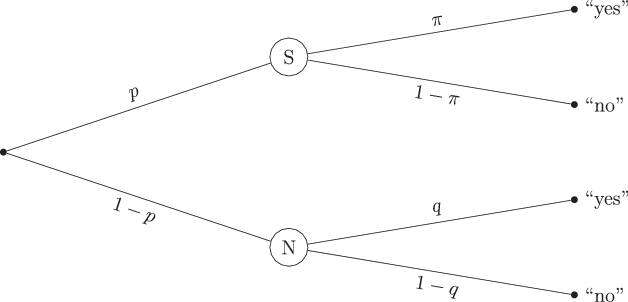
Fig. 3 Probability tree of the unrelated question model.The sample is divided into participants drawing the sensitive question S and those drawing the neutral question N (with the probabilities p and 1−p, respectively). The probability of a yes-answer to the sensitive question is π, for a no-answer it is 1−π. Participants drawing the neutral question answer “yes” or “no” with the probabilities of q and 1−q, respectively
In summary, the model consists of two design parameters, that is, the probabilities p, to be assigned the sensitive question, and q, to answer the neutral question with “yes”, and one unknown parameter of interest, the prevalence π of the sensitive attribute or behavior. The probability of a yes-answer, γ (we renamed this parameter to avoid confusion since it is originally labeled λ like the rate in the Poisson model) is then
6
according to the model. γ can be estimated via the observable relative frequency of yes-answers. With
, π can be estimated by
7
The variance of π is
8
and 95% confidence intervals can be formed by
9
Notably, other than in the Poisson model, π is defined with respect to the time frame posed by the question. Thus, if the question states, “Did you gamble in the last year?”, π refers to the one-year prevalence of gambling (i.e., anyone who gambled during this time), not the proportion of gamblers (i.e., anyone who gambles regularly, independent of the exact time frame). Consequently, like any other RRM, the UQM faces the same problems of ambiguity and inability to estimate rates of occurrence as traditional direct questioning techniques (DQ) when it comes to measuring prevalence of behavior due to time-constrained questions. While multiple authors have already designed RRMs that can be used for sensitive quantitative variables (e.g., Greenberg et al., 1971; Himmelfarb & Edgell, 1980; Huang et al., 2006; Kumar, 2022; Liu & Chow, 1976), these solutions still comprise the problem that those kinds of questions might be more difficult to answer, as explained above.
1.3 The UQMP: A new approach for time-constrained questions on sensitive topics
In this paper, we propose a new approach, combining the benefits of the Poisson model and RRMs, enabling a questioning technique which is both independent of time constraints and valid for questions about sensitive topics. Since the UQM has some qualities that distinguishes it from other RRMs, the paper at hand will focus on this particular model. This is because, for one, the UQM is regarded as more psychologically acceptable than several other RRMs, as already mentioned. Additionally, it is one of the most efficient RRMs (Ulrich et al., 2018).
Our proposed extension of the UQM via the Poisson model — let us call it the UQMP — is depicted in Fig. 4. As can easily be seen when comparing it to the UQM presented in Fig. 3, the proposed UQMP basically extends the classic UQM with the possibility to distinguish carriers from non-carriers, independent of time constraints. Like in the UQM, the probability tree of the UQMP spreads into two main branches. The upper branch represents participants led to the sensitive question, the lower one represents participants getting assigned the neutral question. The lower branch is identical to that of the UQM, leading to the possibilities of participants answering “yes” or “no” (with the probabilities q or 1−q, respectively). However, in the upper branch, the parameter π does not represent the probability of giving a positive answer to the sensitive question, like it is the case in the UQM. Instead, it is defined as the probability that a random participant drawing the sensitive question is a carrier of the researched attribute, like in the Poisson model. From there on out, like in the standard Poisson model, the non-carriers are assumed to always answer “no”, while the carriers might answer either “yes” or “no”, depending on the time frame t that the sensitive question refers to.

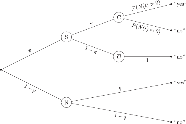
Fig. 4 Probability tree of the Poisson extension of the unrelated question model.The sample is divided into participants drawing the sensitive question S and those drawing the neutral question N (with the probabilities p and 1−p, respectively). The probability of a participant drawing the sensitive question being a carrier C is π, for them being a non-carrier is 1−π. Carriers answer “yes” to the sensitive question with the probability , or “no” with the probability . Non-carriers are assumed to answer “no” in all cases. Participants drawing the neutral question answer “yes” or “no” with the probabilities of q and 1−q, respectively
The probability of a yes-answer to a question referring to the time frame t in the UQMP is
10
with λ representing the average rate of occurrence of the researched behavior, like in the standard Poisson model.
Similar to the Poisson model, we can estimate the parameter values of π and λ by varying the time frames ti that the sensitive question is referring to (the neutral question has to be invariant between groups, so that q is constant). At least two time frames ti are needed for parameter estimation. To test model fit, a third time frame is needed. Additional time frames might be helpful to increase the accuracy of parameter estimation. As in the Poisson model, the maximum likelihood procedure can be used to estimate the parameters (see Supplementary Material).
Differently to the standard Poisson model, the probability P(“yes” |t) is not equivalent to the prevalence curve, since not every yes-answer in the UQMP is related to the topic of interest. Instead, the probability distribution of P(“yes” |t) includes the probability of answering “yes” to the neutral question as well. This can clearly be seen in Fig. 5, since the curve does not start at an intercept of 0, but at
and since the asymptote is not located at π, but at
. Additionally, the slope of the curve is stretched by the parameter p.


Fig. 5 Examples of the probability distribution of P(“yes” |t) as a function of π and λ with varying values for both parameters.The UQM design parameters are set to and , thus the intercept at is located at
Consequently, the prevalence curve must be represented by the conditional probability of answering “yes”, given the sensitive question. This conditional probability is calculated by
11
Inserting the probability of answering “yes” in the UQM procedure (see Eq. 10) yields a function that is equivalent to Eq. 5.
1.4 The study at hand
In this study, we tested the applicability of the proposed model, the UQMP. To do so, we used the UQMP to estimate the prevalence of drinking and driving, defined as “driving while drunk”, in a sample of Germans regularly participating in motorized traffic. Additionally, we applied the standard Poisson model, using a direct question, to measure the same prevalence. Thus, a comparison between the UQMP and the standard Poisson model, using the DQ technique, is enabled. To control whether the UQM method works as intended, we also asked a non-sensitive question in the DQ and UQM format; the prevalence estimates for non-sensitive attributes should not differ between both methods. Finally, we asked some questions regarding the perception of the survey, e.g., if the participants felt anonymous during the survey process.
Only some research exists regarding the prevalence of drinking and driving in Germany. While the German police and the Federal Office for Motorized Traffic publish some statistics about traffic violations involving alcohol, those numbers are not indicative of the true prevalence of drinking and driving. This is because not every person gets caught driving under the influence, thus a substantial dark figure (i.e., the cases not known by the authorities) of drinking and driving is to be assumed. The likely most valid measurement for this dark figure was provided by Krüger and Vollrath (1998), who measured the prevalence with a roadside survey: In cooperation with the police, they pulled drivers over randomly and measured their blood alcohol level. As a result, 1% of the drivers violated the allowed maximum level of blood alcohol concentration (BAC), which is 0.05% according to German law. However, it is still possible that Krüger and Vollrath (1998) underestimated the prevalence of drunk drivers, as some drivers may choose to travel on less-monitored roads after alcohol consumption.
Unfortunately, a more up-to-date roadside survey has not been conducted in Germany since. In a more recent study, Goldenbeld et al. (2020) used direct questions in an online survey to measure the prevalence of drinking and driving in multiple European and non-European countries. For Germany, they found that 9% of drivers admitted that they might have violated the legal BAC-level in the last month. In another study, Iberl (2021) compared the UQM and DQ in an online survey to measure the lifetime prevalence of drinking and driving for German university students, finding no difference between the prevalence estimates in both methods. Drinking and driving was defined similarly as in Goldenbeld et al. (2020), as “driving under the influence of alcohol while accepting the possibility of a rule violation” (Iberl, 2021, p. 277), resulting in an estimation of
. This UQM lifetime prevalence estimate of 0.44 was used as a point of orientation in the study at hand. This prevalence is most likely lower in a student sample compared to the general population, as students are younger and less likely to own motorized vehicles (younger people were also less likely to be drunk drivers in the roadside survey by Krüger & Vollrath, 1998). This could indicate that the proportion of trait carriers would be higher than 0.44 in a more representative sample. However, the definition of drinking and driving in Iberl (2021) is much broader than the one used in our study, which is probably the main reason why the estimate of 0.44 is much higher than in other studies. We therefore assumed that the proportion of true trait carriers should be lower than 0.44 in our sample.
As the non-sensitive question for validating the UQM, we used a question about the eye color of the participants, assuming eye color to be a non-sensitive attribute. To be precise, we estimated the prevalence of blue eye color via the DQ and UQM methods.
Our preregistered hypotheses (see https://osf.io/nh6e9) were:1
- 1.
The proposed model (UQMP) fits the data well. Thus, it might be suitable for application in prevalence research about sensitive topics.
- 2.
(a) The prevalence of drinking and driving (i.e., π) is higher in the UQMP than in the standard Poisson model based on direct questioning, which may indicate a more accurate estimate.
(b) The UQM should result in participants in the first group (UQMP) feeling more anonymous compared to participants in the second group (DQ based on Poisson model).
- 3.
The proportion of trait carriers is expected to be lower than 0.44 (the lifetime prevalence for drinking and driving in students in Iberl, 2021).
- 4.
The prevalence estimate of the non-sensitive eye color question does not differ between questioning via the UQM and via a direct question.
2 Method
2.1 Design
The study at hand is built as a 2 (DQ vs. UQM group) × 4 (drinking and driving in the past week/month/six months/year) between-subjects design. Participants were randomly assigned to one of the eight resulting groups. The questions in the survey were presented in a fixed order for all participants regardless of the group. Quotas regarding age and gender were set in advance. Those were derived from the data of the Kraftfahrt-Bundesamt [Federal Office for Motor Traffic] (2022) and were applied to the aspired sample size set in advance in the preregistration.
2.2 Participants
For our survey, we aimed for a sample representative of regular motorized road users in Germany. To reach this goal, the market research company Bilendi S.A. was commissioned to recruit a sample of
German participants with the same demographic properties as the population of Germans with a driver’s license (see Kraftfahrt-Bundesamt [Federal Office for Motor Traffic], 2022).
The sample size rationale for the study was based on simulations, which in turn, were based on parameter values that seemed realistic. For the number of carriers, we assumed a prevalence of
. This assumption was based on the prevalence in Iberl (2021) and the hypothesis that the π estimate in the study at hand would be smaller due to different wording of the questions posed. For the mean rate of drinking and driving we assumed
(i.e., one instance of drunk driving per month2) to be a somewhat realistic value. Assuming these values, good accuracy for the maximum-likelihood-estimation of both parameters is achieved in the UQMP with a sample size of 600 participants for four groups and time frames ti (past week/month/six months/year; the mean standard deviation for π and λ was 0.021 and 0.244, respectively). For the standard Poisson model, 200 participants per group were sufficient for good estimation accuracy (mean standard deviation of 0.023 for π and 0.231 for λ). In total, the simulations pointed toward a sample size of 3200 participants as adequate. To assure a sufficient sample size after data exclusion, we increased the aspired sample size by 15%, yielding a final goal sample size of 3680 participants.
In total, 5739 potential participants followed the invitation link to the online survey. Participants who did not drive a motor vehicle at least once per week at the time of the study were screened out at the beginning of the survey. 279 participants who failed an implemented attention check were screened out as well (5% of the potential participants). After screen-outs,
completed surveys remained, fulfilling the aspired sample size. Furthermore, we used the relative speed index (RSI) approach of Leiner (2019b) to identify participants who answered the survey substantially faster than average. The RSI was computed according to Leiner (2019b) and calculated separately for each group, to take possible differences in completion time into account. In total, after applying the described and preregistered exclusion criteria (see Iberl et al., 2022a), a sample of
participants remained.
Of the 3529 participants, 1512 or 43% stated their gender as female, 2007 or 57% as male and 10 or 0% as non-binary. The mean age in the sample was 48.9 years (
) with a minimum age of 18 and a maximum age of 89. The distribution of gender and age in the sample matches well with the one for Germans with a driver’s license according to the Kraftfahrt-Bundesamt [Federal Office for Motor Traffic] (2022), see Table 1. Thus, we believe to have achieved a sample approximately representative of the motorized road users in Germany with respect to age and gender (2022).
Table 1 Distribution of demographics in the sample compared to those of the German population owning a driver’s license
| Demographic | Distribution |
Sample (%) | Population (%) |
The reference distribution of demographics is based on data by the Kraftfahrt-Bundesamt [Federal Office for Motor Traffic] |
Gender | Female | 42.8 | 43.1 |
Male | 56.9 | 56.9 |
Non-binary | 0.3 | 0.0 |
Age | 18–29 years | 15.8 | 16.8 |
30–39 years | 19.5 | 20.1 |
40–49 years | 14.1 | 14.2 |
50–59 years | 17.5 | 16.7 |
60 years and older | 33.2 | 31.8 |
2.3 Material and procedure
After preparation of the survey, using the software SoSciSurvey (Leiner, 2019a) and preregistration of the study, the recruitment phase started on July 27th, 2022 via Bilendi S.A. First, the participants received the link to the online questionnaire from the aforementioned market research company. Upon following this link, they were presented an introductory text, explaining the legal framework of the survey (voluntary participation, guarantee of anonymity and contact information of the responsible party). At the same time, conditions for participation were determined (at least 18 years of age and fluency in the German language). Lastly, it was announced that they will be able to create a personal code with which they would be able to delete their data if they wanted to. The participants created this code on the following page.
On the third page, information about demographics was inquired. At later stages of the sampling phase, some of the preset demographic quotas were already fulfilled (e.g., the aspired number of male participants was complete). In this case, any participant of the same demographic (e.g., any male participant) would be screened out after this page and redirected to another website appointed by the market research company. The demographic questions were followed by the question about traffic participation on the next page (“Do you drive a motor vehicle (e.g., a car, motorbike, motor scooter, etc.) at least once per week?”), screening out any participants who drove more rarely than once a week.
Next, the participants were queried about drinking and driving. At this point, it was explained to the UQM group that a specific questioning method would be used in this survey and that this method would guarantee their complete anonymity. On the next page, they were instructed to think about the birth date of a friend or relative and to remember this birth date for the next page. Then, they were presented the UQM question design:
Is the birthday of the person you thought about between the 1st and 10th day of the respective month? Then please answer question A honestly.
Is the birthday of the person you thought about between the 11th and 31st day of the respective month? Then please answer question B honestly.
Question A: Is the birthday of the person you thought about in the first half of the year, so before the 1st July of a year?
Question B: Did you drive a motorized vehicle (a car, motorcycle, scooter, etc.) in the last week/month/six months/year while being drunk or knowing that you had too much to drink?
So, the participants could be led to the neutral Question A or the sensitive Question B about drinking and driving, depending on the birthday they thought of. Then, they should answer honestly, regardless of the question they were led to.
The time frame that Question B referred to varied, depending on the group of participants. The intro question and Question A concerned the birth date the participants were instructed to think about. They were designed so that the probability to be assigned to the sensitive Question B was
and that the probability to answer “yes” to Question A was
.
Meanwhile, participants in the DQ group were told that on the next page, there would be a question regarding drinking and driving, followed by an independent extra question. They were also guaranteed anonymity. After continuing, the DQ group was presented the direct question about drinking and driving. This question was identical to Question B of the UQM design, also with varying time frames depending on group, but posed directly.
Afterwards, it was announced to the participants in the UQM group that another question using the same method, but tackling another topic, would be asked. However, the attention check followed on the next page. In this attention check, participants were asked which one of six cities was not located in Germany. While five of the named cities were German, London was included as the odd one out. Participants who failed to answer the attention check correctly were screened out, as mentioned above.
The attention check was succeeded by the eye color question. The participants in the UQM group were again requested to think about a certain birth date. On the following page, the questions regarding eye color were posed to them in the same way as the question about drinking and driving, but with Question B being worded as “Do you have blue eyes?” (obviously without referring to a time frame). The same question was presented directly to participants in the DQ group after they completed the attention check.
Participants who completed the eye color question were confronted with questions about survey impression on the last page of the survey. These questions inquired, using a five-point Likert scale, how anonymous the participants felt during survey completion and how reprehensible they thought drinking and driving was. Subsequently, participants were redirected to a website of Bilendi S.A.
Completing the survey took the participants in the final sample 3 min and 38 s on average (
). Unsurprisingly, participants in the UQM group took longer on average (3 min and 56 s,
) than participants in the DQ group (2 min and 45 s,
). Data acquisition ended on August 8th, 2022.
3 Results
All computations were executed with the free software R (R Core Team, 2018). See Iberl et al. (2022b) for the complete data and analysis code.
The sample sizes as well as the observed yes- and no-answers to the drinking and driving question are presented in Table 2 for each subgroup. The combined sample sizes are
for the four UQM groups and
for the four DQ groups.
Table 2 Observed frequencies of responses for each subgroup to the question of drinking and driving
Group | Time frame |
| “yes” | “no” |
UQM | One week | 672 | 283 | 389 |
One month | 670 | 272 | 398 |
Six months | 654 | 276 | 378 |
One year | 655 | 277 | 378 |
DQ | One week | 210 | 20 | 190 |
One month | 221 | 23 | 198 |
Six months | 215 | 17 | 198 |
One year | 232 | 22 | 210 |
The prevalence π and mean rate λ for drinking and driving were estimated via the maximum likelihood method both for the UQM group, using the UQMP, and the DQ group, using the standard Poisson model (see Supplementary Material). For reliable calculation of standard errors and 95% confidence intervals, a parametric bootstrapping procedure with 1000 bootstrap samples was employed (see, e.g., Boos, 2003). Table 3 contains the parameter estimates for the UQM group via UQMP and the DQ group via the Poisson model.
Table 3 Maximum likelihood estimates, standard errors, and 95% bootstrap confidence intervals for π and λ, and results of G-tests for the UQMP and the standard Poisson model
Group |
|
|
|
|
Estimate | SE |
| Estimate | SE |
|
The rate of occurrence λ has the dimension [month]−1. The point estimates, standard errors, and confidence intervals were calculated using a parametric bootstrap algorithm with 1000 bootstrap samples. All G-tests were carried out with two degrees of freedom (
). p values are presented for interpretation of the G-tests |
UQM | 0.388 | 0.015 |
| 9.810 | 0.617 |
| 1.855 | 0.173 |
DQ | 0.096 | 0.010 |
| 8.756 | 2.012 |
| 1.041 | 0.308 |
In line with Hypothesis 1, the G-tests are non-significant for both models. As predicted in Hypothesis 2a, the proportion of carriers is considerably higher in the UQMP method. While
in the DQ group, meaning around 10% of the sample can be described as drunk drivers, the estimate resulting in the UQMP is as high as
(but, as expected, lower than 0.44, see Hypothesis 3). The λ-estimates are very high in both groups, which indicates a high rate of drinking and driving among the carriers. But, since the upper boundary of the 95% confidence intervals for λ reach the set upper limit for parameter estimation (10), those estimates are to be interpreted cautiously.
The graphics in Fig. 6 show similar resulting prevalence curves for both the UQMP and the standard Poisson model, with the UQMP’s prevalence curve having a higher asymptote (as determined by
). The curves rise very steeply, reaching the asymptote already on the first point of measurement. This kind of fast-rising curve is a result of the high λ-values estimated in both models. According to these results, carriers of the “drinking and driving”- attribute show this behavior regularly, since its probability of occurrence does not seem to change over time. With a behavioral pattern like this, the specific value of
could theoretically be infinite in the Poisson model, and should thus not be interpreted.

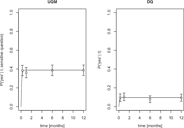
Fig. 6 The prevalence curves for the UQMP and the standard Poisson model resulting from parameter estimation in both methods.The points indicate the prevalence estimates per time frame. The error bars represent 95% confidence intervals
Regarding the control question of eye color, 95% confidence intervals were calculated via the standard procedures for the respective type of question (see Eq. 9) for the UQM group, and the standard binomial 95%-CI for the DQ group. In the UQM group (n = 2651), a prevalence for blue eyes of 0.517 (95% CI [0.489, 0.546]) was estimated. The prevalence in the DQ group (
) is significantly lower with an estimate of 0.355 (95% CI [0.324, 0.387]). Thus, these results contradict Hypothesis 4 regarding the equality of both prevalence measures for eye color.
Most participants, regardless of group, felt that their anonymity was well protected in the survey. On the 5‑point Likert scale, the mean score was 4.213 (
). Still, the feeling of anonymity differed significantly between groups (Welch Two Sample t‑test;
,
), with the UQM group showing slightly higher scores
than the DQ group
. The damnability of drinking and driving was rated highly by both groups (
,
), with no statistically significant differences between mean scores (Welch Two Sample t‑test;
,
). The results of the questions about the participants’ impression of the questionnaire concur with the preregistered Hypothesis 2b.
4 Discussion
In this paper, we presented a novel method, the UQMP, combining the Poisson model (Iberl & Ulrich, 2023) with the unrelated question model by Greenberg et al. (1969).
Through the approach of the Poisson model, unambiguous prevalence estimation and the estimation of the mean rate of a behavior’s occurrence are rendered possible. Additionally, the UQM is designed to solve the problem of socially desirable answers to sensitive questions by providing the participants with complete and transparent anonymity. The model was applied to the sensitive topic of drinking and driving in motorized traffic, and compared to the Poisson model, another recently proposed method (Iberl & Ulrich, 2023). For this purpose, a sample representative of German drivers in terms of gender and age was queried via an online survey. Although the model appears to fit the data based on the G-tests, the obtained flat prevalence curves were unexpected based on this model. Thus, Hypothesis 1 can only be conditionally confirmed. Regarding the proportion of trait carriers, we get an estimate as high as 39% for drunk drivers in Germany using the UQMP. With direct questioning, in the standard Poisson model, the amount of carriers is estimated to be lower, as expected (see Hypothesis 2a), with 10% of the participants being identified as carriers. As anticipated, these percentages are lower than the 44% lifetime-prevalence that resulted for drinking and driving in the student survey of Iberl (2021) (see Hypothesis 3). Also, evidence is found for participants in the UQMP group to feel somewhat more protected regarding their anonymity, compared to the DQ group (see Hypothesis 2b). An unexpected result can be found in the neutral question about eye color (Hypothesis 4): While we assumed no difference in estimation for blue eye prevalence between UQM and DQ methods, the results differ significantly.
In the following, we will first interpret the values resulting from the parameter estimations in the Poisson model and the UQMP methods. Then, we discuss the unexpected results in the blue eye color prevalence estimation, proposing some possible explanations and summarizing the results of a follow-up study we conducted to test one of those explanations. Afterwards, we conclude the applicability of the UQMP. We finish the discussion with an assessment of our findings and possible further research regarding the uses of the Poisson model.
4.1 Comparing the Poisson model and the UQMP
Interestingly, the prevalence curves for both the standard Poisson model and the UQMP are similar in shape, rising very steeply and reaching the asymptote already on the first point of measurement (one week). In turn, the λ parameters assume very high values in both models, with 9.810 for the UQM group and 8.756 for the DQ group. However, as mentioned above, both 95% confidence intervals include the preset upper limit for estimation, thus the values can not be interpreted as the amount of times the behavior occurred in the reference time unit (in this case, one month). This is a consequence of all four measurement points, in both groups, yielding the same relative frequency of yes-answers. Thus, the data truly support a straight line for a prevalence curve, instead of an actual curve. With such a result, theoretically, λ could be infinite.
When it comes to behaviors like drinking and driving, one would expect to see a concave prevalence curve, meaning that the proportion of people engaging in the behavior should increase with the length of the time frame. Due to this, the rather flat prevalence curves found in this study are surprising. One possible explanation for the unexpected curves is that many participants may have misread or misunderstood the questions, resulting in equal proportions of yes-answers regardless of the time frame. Some studies (see e.g., Lannoy et al., 2021; Maurage et al., 2020; National Institute of Alcohol Abuse and Alcoholism [NIAAA], 2018) have identified binge drinkers, who consume large amounts of alcohol on rare occasions. This also suggests that the prevalence curve for drinking and driving should indeed be concave (especially with past-month-prevalence estimates as high as 26%, see National Institute of Alcohol Abuse and Alcoholism [NIAAA], 2018). However, binge drinkers might not drive during their times of consumption, which would not have influenced our measurement of drinking and driving prevalence. While the validity of the resulting prevalence curves remains unclear, such flat functions can be compatible with the model’s assumptions: If drinking and driving occurs very regularly for some individuals, at least once a week, while the rest of the population does not engage in this behavior, flat prevalence curves would be expected in the Poisson model.
According to the UQMP, the carriers account for 39% of the sample, while the π estimate for the standard Poisson model is much lower with around 10%. Thus, our DQ estimation for Germans who drive under the influence is remarkably close to the one of Goldenbeld et al. (2020), who found a 30-days-prevalence of 9%, also by DQ. The much higher prevalence of carriers resulting from the UQMP could theoretically indicate a more valid estimation since some respondents in the DQ group might not have answered truthfully due to social desirability bias. The results in the eye color question, however, clearly point towards problems with overestimation in the UQM group.
4.2 Unexpected results: Blue eye color prevalence
The expectation for estimation of blue eye color prevalence was for both methods to yield the same results (Hypothesis 4). Since this question should not be perceived as sensitive, no social desirability bias should influence the answers, resulting in equal prevalence estimates for the UQM and DQ groups. The value of 52% blue-eyed respondents resulting for the UQM group not only seems high compared to the 36% in the DQ group, but also when looking at the (sparse) corresponding literature. In a 19th-century study of Virchow, which has been deemed still relevant by Katsara and Nothnagel (2019), a prevalence of almost 40% for blue eyes in the German population was found. On a German website about “rapid facts”, a non-published study is cited to have found a prevalence of 30% for blue eyes in Germany; additionally, the users of the website can report their own eye color, resulting in a prevalence of 31% (kurzwissen.de, 2019). While the latter source is of questionable validity, it also points towards our UQM estimate being too high and towards the DQ estimate as the more valid one. Regardless of the actual prevalence, the difference between both methods’ estimates is unexpected. The most logical explanation seems to be an unknown effect related to the questioning technique used in both groups.
There are multiple possible explanations for how a supposed effect of the questioning technique could have come to pass. First, since we did not randomize the order of the alcohol-related and eye-color-related questions, some kind of order effect could explain the results. Maybe the participants in the UQM group did not pay as much attention to the instructions after they already answered both the question about drinking and driving and the attention check. Or maybe the birth date they thought about while answering the first question influenced the birth date they used for the second question about eye color, distorting the design probabilities of p and q. Either way, if the position of the eye color question caused the suspected inflation in the prevalence estimate of blue eye color, the question regarding drinking and driving could be unaffected by this, since it was asked before. To test this explanation of order effects, we conducted a follow-up a study using the curtailed sampling approach (Reiber, Schnuerch, & Ulrich, 2022; Wetherill, 1975). In this follow-up study, we switched the order of the UQM questions, asking the eye color question before the attention check and the drinking and driving question. If the possible order effect caused the high value for blue eye color prevalence in the UQM group, an estimate in the realm of the value in the DQ group, 36%, should be expected. However, the follow-up study led to an estimate for blue eye prevalence via UQM similar to the one of 52% in the main study, even though the questions’ positioning was swapped. So, order effects alone do not seem to have influenced the results of the neutral question, pointing towards different explanations (for a more detailed description of the follow-up study see Iberl, Aljovic, Ulrich, Reiber (2022c) and the Supplementary Material).
A second possible explanation lies in some kind of random responding by the participants (independent of the order of questions). Some respondents might not follow the instructions thoroughly enough (either by unwillingness or due to comprehension issues), in turn answering randomly. This would, of course, influence not only the neutral question of eye color, but also the results for the prevalence of drinking and driving in the UQM group. To test this explanation post-hoc, we calculated, assuming the true prevalence of blue eye color to be 36% like in the DQ group, how many participants would have to answer “yes” randomly (with the probability of 0.5) in order to produce the result of 52%. Surprisingly, more than 100% of randomly responding participants would be needed for this result to occur. So, a truly random pattern of responding can not be the only reason for the unexpected results. The explanation gets more likely if one assumes a non-equal distribution for the probabilities of “randomly” answering “yes” or “no”. Potentially, the yes-answer is chosen more often than the no-answer in random responding (because it is more appealing for some reason or just because it is read first). If we assume a probability of random yes-answers of 0.75, about one-third of the participants would have to respond randomly to get our result for blue eye prevalence. This seems more plausible than random responding with equal probabilities for yes- and no-answers. But, even if we assume an uneven probability for both answers, random responding by itself seems to be unlikely as an explanation for the results. A recent study by Meisters et al. (2022) supports this claim, finding that while random responding exists in the researched RRM, it only has a minor influence on the resulting prevalence. However, there also seems to be some contrary evidence pointing towards random responding as a substantial factor in RRMs (Walzenbach & Hinz, 2019).
A third explanation could lie in the nature of the surveyed sample. Since the sample consisted of most likely highly experienced participants in regards to online surveys, it is reasonable to assume that privacy concerns were less common compared to the general population. This is supported by the result that the participants in the DQ group felt almost as anonymous as those in the UQM group. As some studies show, RRMs work best when the question is perceived as sensitive, so when a social desirability bias is to be expected when using DQ instead (e.g., Lensvelt-Mulders et al., 2005; Tourangeau & Yan, 2007). With highly survey-experienced participants who feel very anonymous, a substantial social desirability bias might be less likely. So, for this specific sample, the UQM might only be perceived as confusing and annoying, instead of a protective question design, leading to the unexpected results through random responding or even noncompliance. Generally, it could be a problem of RRM application in online surveys that it is hard to control whether the participants comprehend the instructions of the method or whether they understand that the RRM provides a high level of anonymity. Unfortunately, it is not yet well understood what role comprehension plays for the validity of RRMs (e.g., Bullek et al., 2017; Hoffmann et al., 2017; Höglinger & Jann, 2018; Meisters et al., 2020). Thus, it may be crucial to conduct RRT surveys in person, with interviewers explaining the procedure to respondents before running the UQM survey (e.g., Striegel et al., 2010).
Multiple other explanations are imaginable as well. For example, the eye color question might not be as neutral as supposed, or it might have been difficult to answer for participants with ambiguous eye colors (like “blue-green” or “grey-blue”), leading to unforeseen response behavior. However, none of these possible effects would seem strong enough to explain the high prevalence of 52% on its own, but some of them might contribute to an inflation of the estimate. So, although we can not identify a single explanation, we might have identified some possible effects that could have caused the high estimate in the UQM group. Regardless, the UQM method seems to be the cause of this inflated estimate. While we can not exclude the reasons to be of a nature regarding the content of the eye color question, which would not influence the estimation for drinking and driving by UQM, we can also not confidently assume the UQM to have worked as intended. Consequently, the DQ estimate seems to be the more accurate result, and the UQMP estimate should be viewed with caution. This, however, is due to the UQM—and not due to the Poisson model used in combination.
In future research, one could test the combination of the Poisson model with different RRMs, such as the crosswise model (CWM, Yu et al., 2008). These combinations would be easy to realize and might yield more plausible results.
5 Conclusion
Albeit we can not rule out problems of the UQM method in view of our findings, the Poisson model seems to work as intended. While the resulting prevalence curves are unexpected in shape, this is caused by the answers of the participants, showing no variation of the proportion of yes-answers between time-frames. Also, the π estimate for drunk drivers resulting by DQ is similar to the results of another study using DQ to measure prevalence of drinking and driving in Germany (Goldenbeld et al., 2020). Additionally, even though the λ estimate seems off at first glance, it behaves as expected given there is no variance between the proportion of yes-answers in the four points of measurement. A “prevalence line” of some sort between the four points of measurement, as resulted in this study, does not contradict the model’s core assumptions: If there exists only a rather small population of carriers that is showing the behavior very frequently, a line is to be expected. To be precise, if the behavior’s rate of occurrence is as high or higher than 1/t1, with t1 being the time frame of the first point of measurement (here: one week), prevalence curves like those in Fig. 6 are likely. This applies to both the Poisson model and the UQMP. Unfortunately, in case of drinking and driving, a shorter reference time frame than one week would probably not have been suitable for usage in the questionnaire. This is because driving under the influence is supposed to be more frequent during the weekend, especially weekend nights, according to some studies (e.g., Krüger & Vollrath, 1998; Vanlaar, 2005). Thus, the assumption of drinking and driving as a Poisson-distributed variable might be invalid for time frames smaller than one week. Regardless of the assumed overestimation due to unforeseen bias caused by the UQM method, the form of the UQM prevalence curve is similar to the one in the DQ group. In these cases, the estimated value for the λ parameter should not be interpreted. Instead, the rate of occurrence of the researched behavior can be assumed to be at least 1 referring to t1, that is, once a week.
To sum up the results of our study regarding the problem of alcohol in motorized traffic, we found that at least 10% of drivers in Germany are frequently, at least once a week, driving under the influence of alcohol. The other (at maximum) 90%, on the other hand, seem to be non-carriers, who essentially never engage in drinking and driving. While the UQMP estimation does not seem reliable, we can not rule out an underestimation of drinking and driving by the standard Poisson model using the DQ method, so the proportion of 10% for drunk drivers can be seen as a lower border for the true amount of carriers. A substantial part of those carriers can be assumed to be participants with problematic or even pathological alcohol consumption. This claim is supported by an older study by Selzer and Barton (1977), which showed that about two-thirds of the drunk drivers in their sample were pathological drinkers. Also, this hypothesis seems valid due to the high amount of problematic drinkers in Germany: According to Atzendorf et al. (2019), 18% of a sample of 9267 Germans between the age of 18 and 64 years reported the use of alcohol in hazardous quantities for the time frame of 30 days before the survey. It stands to reason to assume that many people with such high alcohol usage still rely heavily on motorized traffic in their everyday lives, as this is generally by far the most used form of transportation in Germany (Bundesministerium für Digitales und Verkehr [Federal Ministry for Digital and Transport], 2021). The fact that the majority of the German population uses a car or another motorized vehicle to commute to their workplace, school or university seems particularly relevant in this context (Bundesministerium für Digitales und Verkehr [Federal Ministry for Digital and Transport], 2021).
In conclusion, the Poisson model used in our study seems suited for practical application, even if the shape of the resulting prevalence curve contradicts this statement at first glance. Still, the Poisson model should be tested and compared with traditional methods in future studies to determine when it is suited best. Furthermore, we showed that the Poisson model can be combined with indirect questioning techniques such as the UQM. There are still open questions regarding the validity of the UQM and RRMs in general, as we have to assume an unexpected inflation of false-positive yes-answers due to the results of our control question about eye color prevalence. Thus, more research is needed to understand the validity of RRMs further and to identify scenarios of when RRMs are (not) to be preferred over DQ methodology. Plus, while the sample size needed for a satisfactory level of statistical power is already high in RRMs compared to DQ, the additional participants needed for implementing a Poisson extension to an RRM is considerable. In further studies, it might be reasonable to test Poisson model extensions and their applicability for different RRMs, like the cheater detection model (CDM, Clark & Desharnais, 1998) or the crosswise model (CWM, Yu et al., 2008). Since they enable time-independent prevalence estimation for objectively anonymous survey procedures, Poisson model extensions for RRMs might be worth the effort.
1 Supplementary Information
Appendix Acknowledgements
We thank an anonymous reviewer for many constructive and detailed comments.
References
Aljovic, A. (2022). Zeitunabhängige Prävalenzschätzung von Alkohol am Steuer: Eine Einführung des Unrelated Question Models mit Poisson-Erweiterung [Time-independent prevalence estimation of drinking and driving: An introduction of the Poisson extension to the Unrelated Question Model]. Unpublished master thesis. →
Aarts, H., & Dijksterhuis, A. (1999). How often did I do it? Experienced ease of retrieval and frequency estimates of past behavior. Acta Psychologica, 103(1–2), 77–89. https://doi.org/10.1016/S0001-6918(99)00035-9. →
Andrie, E. K., Tzavara, C. K., Tzavela, E., Richardson, C., Greydanus, D., Tsolia, M., & Tsitsika, A. K. (2019). Gambling involvement and problem gambling correlates among European adolescents: Results from the European Network for Addictive Behavior study. Social Psychiatry and Psychiatric Epidemiology, 54(11), 1429–1441. https://doi.org/10.1007/s00127-019-01706-w. a, b, c
Atzendorf, J., Rauschert, C., Seitz, N.-N., Lochbühler, K., & Kraus, L. (2019). The use of alcohol, tobacco, illegal drugs and medicines: An estimate of consumption and substance-related disorders in Germany. Deutsches Ärzteblatt International, 116(35–36), 577–584. https://doi.org/10.3238/arztebl.2019.0577. a, b
Beck, F., Léger, D., Fressard, L., Peretti-Watel, P., Verger, P., & Group, C. (2021). Covid-19 health crisis and lockdown associated with high level of sleep complaints and hypnotic uptake at the population level. Journal of Sleep Research, 30(1), e13119. https://doi.org/10.1111/jsr.13119. →
Birkel, C., Church, D., Erdmann, A., Hager, A., & Leitgöb-Guzy, N. (2022). Sicherheit und Kriminalität in Deutschland – SKiD 2020: Bundesweite Kernbefunde des Viktimisierungssurvey des Bundeskriminalamts und der Polizeien der Länder. https://www.bka.de/DE/UnsereAufgaben/Forschung/ForschungsprojekteUndErgebnisse/Dunkelfeldforschung/SKiD/Ergebnisse/Ergebnisse_node.html [Safety and crime in Germany—SKiD 2020: Nationwide findings of the Victimization Survey by the German Federal Office of Criminal Investigation and by the Police of the federal states]. →
Boos, D. D. (2003). Introduction to the bootstrap world. Statistical Science, 18(2), 168–174. https://doi.org/10.1214/ss/1063994971. →
Boruch, R. F. (1971). Assuring confidentiality of responses in social research: a note on strategies. The American Sociologist, 27701807, 308–311. →
Bousfield, W. A., & Sedgewick, C. H. W. (1944). An analysis of sequences of restricted associative responses. The Journal of General Psychology, 30(2), 149–165. https://doi.org/10.1080/00221309.1944.10544467. →
Bullek, B., Garboski, S., Mir, D. J., & Peck, E. M. (2017). Towards understanding differential privacy: When do people trust randomized response technique? Proceedings of the 2017 CHI Conference on Human Factors in Computing Systems. (pp. 3833–3837). https://doi.org/10.1145/3025453.3025698. →
Bundesministerium für Digitales und Verkehr [Federal Ministry for Digital and Transport] (2021). Verkehr in Zahlen 2021/2022 [Traffic in numbers 2021/2022]. https://bmdv.bund.de/SharedDocs/DE/Publikationen/G/verkehr-in-zahlen-2021-2022-pdf.pdf?__blob=publicationFile a, b
Burr, M. L., Butland, B., King, S., & Vaughan-Williams, E. (1989). Changes in asthma prevalence: two surveys 15 years apart. Archives of Disease in Childhood, 64(10), 1452–1456. https://doi.org/10.1136/adc.64.10.1452. →
Clark, S. J., & Desharnais, R. A. (1998). Honest answers to embarrassing questions: detecting cheating in the randomized response model. Psychological Methods, 3(2), 160–168. https://doi.org/10.1037/1082-989X.3.2.160. →
Cullen, K. A., Ambrose, B. K., Gentzke, A. S., Apelberg, B. J., Jamal, A., & King, B. A. (2018). Notes from the field: Use of electronic cigarettes and any tobacco product among middle and high school students—United States, 2011–2018. Morbidity and Mortality Weekly Report, 67(45), 1276–1277. https://doi.org/10.15585/mmwr.mm6745a5. →
de kurzwissen (2019). Augenfarben Häufigkeit in Deutschland & weltweit [Eye colour prevalence in Germany & worldwide]. kurzwissen.de. https://kurzwissen.de/augenfarben-haeufigkeit/ →
Dietz, P., Iberl, B., Schuett, E., van Poppel, M., Ulrich, R., & Sattler, M. C. (2018). Prevalence estimates for pharmacological neuroenhancement in Austrian university students: Its relation to health-related risk attitude and the framing effect of caffeine tablets. Front. Pharmacol., 9(494), 1–9. https://doi.org/10.3389/fphar.2018.00494. →
Echterhoff, G., & Hirst, W. (2006). Thinking about memories for everyday and shocking events: Do people use ease-of-retrieval cues in memory judgments? Memory & Cognition, 34(4), 763–775. https://doi.org/10.3758/BF03193424. →
Ferrante, T., Castellini, P., Abrignani, G., Latte, L., Russo, M., Camarda, C., Veronesi, L., Pasquarella, C., Manzoni, G. C., & Torelli, P. (2012). The pace study: Past-year prevalence of migraine in parma’s adult general population. Cephalalgia, 32(5), 358–365. https://doi.org/10.1177/0333102411434811. →
Fiedler, K., & Schwarz, N. (2016). Questionable research practices revisited. Social Psychological and Personality Science, 7(1), 45–52. https://doi.org/10.1177/1948550615612150. →
Goldenbeld, C., Torfs, K., Vlakveld, W., & Houwing, S. (2020). Impaired driving due to alcohol or drugs: International differences and determinants based on E‑Survey of Road Users’ Attitudes first-wave results in 32 countries. IATSS Research, 44(3), 188–196. https://doi.org/10.1016/j.iatssr.2020.07.005. a, b, c, d
Greenberg, B. G., Abul-Ela, A.-L. A., Simmons, W. R., & Horvitz, D. G. (1969). The unrelated question randomized response model: theoretical framework. Journal of the American Statistical Association, 64(326), 520–539. a, b
Greenberg, B. G., Kuebler Jr, R. R., Abernathy, J. R., & Horvitz, D. G. (1971). Application of the randomized response technique in obtaining quantitative data. Journal of the American Statistical Association, 66(334), 243–250. https://doi.org/10.2307/2283916. →
Han, B., Compton, W. M., Gfroerer, J., & McKeon, R. (2015). Prevalence and correlates of past 12-month suicide attempt among adults with past-year suicidal ideation in the united states. The Journal of Clinical Psychiatry, 76(3), 15414. https://doi.org/10.4088/JCP.14m09287. →
Himmelfarb, S., & Edgell, S. E. (1980). Additive constants model: A randomized response technique for eliminating evasiveness to quantitative response questions. Psychological Bulletin, 87(3), 525. https://doi.org/10.1037/0033-2909.87.3.525. →
Hoffmann, A., Waubert de Puiseau, B., Schmidt, A. F., & Musch, J. (2017). On the comprehensibility and perceived privacy protection of indirect questioning techniques. Behavior Research Methods, 49, 1470–1483. https://doi.org/10.3758/s13428-016-0804-3. →
Höglinger, M., & Jann, B. (2018). More is not always better: An experimental individual-level validation of the randomized response technique and the crosswise model. PLOS ONE, 13(8), e201770. https://doi.org/10.1371/journal.pone.0201770. →
Höglinger, M., Jann, B., & Diekmann, A. (2016). Sensitive questions in online surveys: an experimental evaluation of different implementations of the randomized response technique and the crosswise model. Survey Research Methods, 10(3), 171–187. https://doi.org/10.18148/srm/2016.v10i3.6703. →
Huang, K.-C., Lan, C.-H., & Kuo, M.-P. (2006). Estimation of sensitive quantitative characteristics in randomized response sampling. Journal of Statistics and Management Systems, 9(1), 27–35. https://doi.org/10.1080/09720510.2006.10701191. →
Iberl, B. (2021). Ein, zwei Bier und ab ans Lenkrad? – Prävalenzschätzung von Alkohol am Steuer durch das Unrelated Question Model [One or two drinks before going for a ride?—Prevalence estimation of driving under the influence via the unrelated question model]. Kriminologie – Das Online-Journal [Criminology-The Online Journal]. https://doi.org/10.18716/ojs/krimoj/2021.3.5. a, b, c, d, e, f
Iberl, B., & Ulrich, R. (2023). On estimating the frequency of a target behavior from time-constrained yes/no survey questions: a parametric approach based on the Poisson process. Psychological Methods. https://doi.org/10.1037/met0000588. a, b, c, d, e, f
Iberl, B., Aljovic, A., Ulrich, R., & Reiber, F. (2022a). Application of a Poisson extension of the unrelated question model to drinking and driving [OSF preregistration]. https://doi.org/10.17605/OSF.IO/NH6E9. →
Iberl, B., Aljovic, A., Ulrich, R., & Reiber, F. (2022b). Application of a Poisson extension of the Unrelated Question Model to drinking and driving [OSF Project with data and code files]. https://osf.io/5pkm4/ →
Iberl, B., Aljovic, A., Ulrich, R., & Reiber, F. (2022c). Follow-up study to “application of a Poisson extension of the unrelated question model to drinking and driving”—testing for possible order effects [OSF preregistration]. https://doi.org/10.17605/OSF.IO/ZV63D. →
Isolauri, J., & Laippala, P. (1995). Prevalence of symptoms suggestive of gastroesophageal reflux disease in an adult population. Annals of Medicine, 27(1), 67–70. https://doi.org/10.3109/07853899509031939. →
Janssen, J., Müller, P. A., & Greifeneder, R. (2011). Cognitive processes in procedural justice judgments: the role of ease-of-retrieval, uncertainty, and experience. Journal of Organizational Behavior, 32(5), 726–750. https://doi.org/10.1002/job.700. →
Katsara, M.-A., & Nothnagel, M. (2019). True colors: a literature review on the spatial distribution of eye and hair pigmentation. Forensic Science International: Genetics, 39, 109–118. https://doi.org/10.1016/j.fsigen.2019.01.001. →
Kraftfahrt-Bundesamt [Federal Office for Motor Traffic] (2022). Fahrerlaubnisbestand im ZFER (Zentrales Fahrerlaubnis-Register) 2022 [Registry of driver’s licenses in the CDLR (Central Driver’s License Registry) 2022]. https://www.kba.de/DE/Statistik/Kraftfahrer/Fahrerlaubnisse/Fahrerlaubnisbestand/fahrerlaubnisbestand_node.html a, b, c, d
Krüger, H.-P., & Vollrath, M. (1998). Fahren unter Alkohol in Deutschland: Die Ergebnisse des Deutschen Roadside Surveys [Driving under the influence in Germany: The results of the German roadside survey]. In H.-P. Krüger (Ed.), Fahren unter Alkohol in Deutschland [Driving under the influence in Germany] (pp. 33–57). Gustav Fischer. a, b, c, d
Krumpal, I. (2013). Determinants of social desirability bias in sensitive surveys: a literature review. Quality & Quantity, 47(4), 2025–2047. https://doi.org/10.1007/s11135-011-9640-9. →
Kumar, A. (2022). Estimation of means of two quantitative sensitive variables using randomized response. Computational Statistics and Applications. https://doi.org/10.5772/intechopen.101269. →
Lannoy, S., Duka, T., Carbia, C., Billieux, J., Fontesse, S., Dormal, V., Gierski, F., López-Caneda, E., Sullivan, E. V., & Maurage, P. (2021). Emotional processes in binge drinking: a systematic review and perspective. Clinical Psychology Review, 84, 101971. https://doi.org/10.1016/j.cpr.2021.101971. →
Leiner, D. J. (2019a). SoSci Survey (Version 3.1.06) [Computer software]. https://www.soscisurvey.de →
Leiner, D. J. (2019b). Too fast, too straight, too weird: non-reactive indicators for meaningless data in internet surveys. Survey Research Methods, 13(3), 229–248. https://doi.org/10.18148/srm/2019.v13i3.7403. a, b
Lensvelt-Mulders, G. J., Hox, J. J., Van der Heijden, P. G., & Maas, C. J. (2005). meta-analysis of randomized response research: thirty-five years of validation. Sociological Methods & Research, 33(3), 319–348. https://doi.org/10.1177/0049124104268664. →
Linton, S. J., Hellsing, A.-L., & Halldén, K. (1998). A population-based study of spinal pain among 35-45-year-old individuals: prevalence, sick leave, and health care use. Spine, 23(13), 1457–1463. →
Liu, P., & Chow, L. (1976). A new discrete quantitative randomized response model. ACM SIGSIM Simulation Digest, 7(3), 30–31. https://doi.org/10.1145/1102746.1102750. →
Maurage, P., Lannoy, S., Mange, J., Grynberg, D., Beaunieux, H., Banovic, I., Gierski, F., & Naassila, M. (2020). What we talk about when we talk about binge drinking: Towards an integrated conceptualization and evaluation. Alcohol and Alcoholism, 55(5), 468–479. https://doi.org/10.1093/alcalc/agaa041. →
McCabe, S. E., Cranford, J. A., & Boyd, C. J. (2006). The relationship between past-year drinking behaviors and nonmedical use of prescription drugs: Prevalence of co-occurrence in a national sample. Drug and Alcohol Dependence, 84(3), 281–288. https://doi.org/10.1016/j.drugalcdep.2006.03.006. →
McKetin, R., McLaren, J., Lubman, D. I., & Hides, L. (2006). The prevalence of psychotic symptoms among methamphetamine users. Addiction, 101(10), 1473–1478. https://doi.org/10.1111/j.1360-0443.2006.01496.x. →
Meisters, J., Hoffmann, A., & Musch, J. (2020). Can detailed instructions and comprehension checks increase the validity of crosswise model estimates? PLOS ONE, 15(6), e235403. https://doi.org/10.1371/journal.pone.0235403. →
Meisters, J., Hoffmann, A., & Musch, J. (2022). More than random responding: empirical evidence for the validity of the (extended) crosswise model. Behavior Research Methods. https://doi.org/10.3758/s13428-022-01819-2. →
Miller, C., Ettridge, K., Wakefield, M., Pettigrew, S., Coveney, J., Roder, D., Durkin, S., Wittert, G., Martin, J., & Dono, J. (2020). Consumption of sugar-sweetened beverages, juice, artificially-sweetened soda and bottled water: An Australian population study. Nutrients, 12(3), 817. https://doi.org/10.3390/nu12030817. →
Molinaro, S., Benedetti, E., Scalese, M., Bastiani, L., Fortunato, L., Cerrai, S., Canale, N., Chomynova, P., Elekes, Z., Feijão, F., et al. (2018). Prevalence of youth gambling and potential influence of substance use and other risk factors throughout 33 European countries: first results from the 2015 ESPAD study. Addiction, 113(10), 1862–1873. https://doi.org/10.1111/add.14275. →
National Institute of Alcohol Abuse and Alcoholism [NIAAA] (2018). Alcohol facts and statistics. Report. https://www.niaaa.nih.gov/sites/default/files/AlcoholFactsAndStats.pdf a, b
Nederhof, A. J. (1985). Methods of coping with social desirability bias: a review. European Journal of Social Psychology, 15(3), 263–280. https://doi.org/10.1002/ejsp.2420150303. →
R Core Team (2018). R: a language and environment for statistical computing. Vienna: R Foundation for Statistical Computing. https://www.R-project.org/ →
Reiber, F., Pope, H., & Ulrich, R. (2020). Cheater detection using the unrelated question model. Sociological Methods & Research. https://doi.org/10.1177/0049124120914919. →
Reiber, F., Bryce, D., & Ulrich, R. (2022). Self-protecting responses in randomized response designs: a survey on intimate partner violence during the coronavirus disease 2019 pandemic. Sociological Methods & Resarch. https://doi.org/10.1177/00491241211043138. →
Reiber, F., Schnuerch, M., & Ulrich, R. (2022). Improving the efficiency of surveys with randomized response models: a sequential approach based on curtailed sampling. Psychological Methods, 27(2), 198–211. https://doi.org/10.1037/met0000353. →
Şaşmaz, T., Öner, S., Kurt, A. Ö., Yapıcı, G., Yazıcı, A. E., Buğdaycı, R., & Şiş, M. (2014). Prevalence and risk factors of internet addiction in high school students. The European Journal of Public Health, 24(1), 15–20. https://doi.org/10.1093/eurpub/ckt051. →
Sawyer, A. N., Smith, E. R., & Benotsch, E. G. (2018). Dating application use and sexual risk behavior among young adults. Sexuality Research and Social Policy, 15(2), 183–191. https://doi.org/10.1007/s13178-017-0297-6. →
Schwarz, N., Bless, H., Strack, F., Klumpp, G., Rittenauer-Schatka, H., & Simons, A. (1991). Ease of retrieval as information: another look at the availability heuristic. Journal of Personality and Social psychology, 61(2), 195. https://doi.org/10.1037/0022-3514.61.2.195. →
Seitz, N.-N., Rauschert, C., Atzendorf, J., & Kraus, L. (2020). IFT-Berichte Bd. 190: Berlin, Hessen, Nordrhein-Westfalen, Sachsen und Thüringen. Ergebnisse des Epidemiologischen Suchtsurvey 2018. München: Institut für Therapieforschung. [IFT-Reports Vol. 190: Substance use and substance use disorders in Berlin, Hesse, North Rhine-Westphalia, Saxony and Thuringia. Results of the 2018 Epidemiological Survey of Substance Abuse] →
Selzer, M. L., & Barton, E. (1977). The drunken driver: a psychosocial study. Drug and Alcohol Dependence, 2(4), 239–253. https://doi.org/10.1016/0376-8716(77)90002-3. →
Soga, M., Evans, M. J., Tsuchiya, K., & Fukano, Y. (2021). A room with a green view: the importance of nearby nature for mental health during the COVID-19 pandemic. Ecological Applications, 31(2), e2248. https://doi.org/10.1002/eap.2248. →
Striegel, H., Ulrich, R., & Simon, P. (2010). Randomized response estimates for doping and illicit drug use in elite athletes. Drug and Alcohol Dependence, 106(2–3), 230–232. https://doi.org/10.1016/j.drugalcdep.2009.07.026. →
Tourangeau, R., & Yan, T. (2007). Sensitive questions in surveys. Psychological Bulletin, 133(5), 859–883. https://doi.org/10.1037/0033-2909.133.5.859. →
Ulrich, R., Pope, H. G., Cléret, L., Petróczi, A., Nepusz, T., Schaffer, J., Kanayama, G., Comstock, R. D., & Simon, P. (2018). Doping in two elite athletics competitions assessed by randomized-response surveys. Sports Medicine, 48(1), 211–219. https://doi.org/10.1007/s40279-017-0765-4. a, b
Vanlaar, W. (2005). Drink driving in Belgium: results from the third and improved roadside survey. Accident Analysis & Prevention, 37(3), 391–397. https://doi.org/10.1016/j.aap.2004.12.001. →
Virudachalam, S., Long, J. A., Harhay, M. O., Polsky, D. E., & Feudtner, C. (2014). Prevalence and patterns of cooking dinner at home in the USA: National Health and Nutrition Examination Survey (NHANES) 2007–2008. Public Health Nutrition, 17(5), 1022–1030. https://doi.org/10.1017/S1368980013002589. →
Walzenbach, S., & Hinz, T. (2019). Pouring water into wine: revisiting the advantages of the crosswise model for asking sensitive questions. Survey Methods: Insights from the Field. https://doi.org/10.13094/SMIF-2019-00002. →
Warner, S. L. (1965). Randomized response: a survey technique for eliminating evasive answer bias. Journal of the American Statistical Association, 60(309), 63–69. →
Wetherill, G. B. (1975). Sequential methods in statistics (2nd edn.). Chapman and Hall. →
Yu, J.-W., Tian, G.-L., & Tang, M.-L. (2008). Two new models for survey sampling with sensitive characteristic: Design and analysis. Metrika, 67(3), 251–263. https://doi.org/10.1007/s00184-007-0131-x. a, b